Learnable Wavelet Transform

Author: [达克寿司]

Original Link: https://zhuanlan.zhihu.com/p/2018421854524688328

In the previous post (link), we discussed wavelet kernel selection. In this article, we go one step further: should we simply choose a common predefined wavelet, or should we train a learnable wavelet? Is it reasonable that different datasets prefer different wavelets? Do trained wavelets differ across datasets? If we train on the same dataset multiple times, do we converge to similar learned wavelets? This post explores these questions with learnable wavelets.

There are two major ideas behind learnable wavelets: one is a meta-learning recommendation system across datasets, and the other is a model that directly treats wavelet kernel coefficients as trainable parameters:

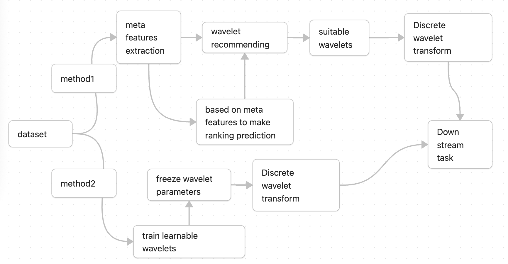
Figure 0: Two learnable wavelet transform approaches

However, before implementing the methods above, we first need to verify whether dataset-adaptive wavelet parameters are actually reasonable. A clustering study can help answer this. Pseudocode:

metrics_list = []
for data in datasets: # iterate over UCR time-series classification datasets
    for wavelet in wavelets: # iterate over discrete wavelet kernels
       coef = DWT(data, level=3) # DWT: discrete wavelet transform; level=3 means three decomposition levels
       metrics (Sparsity,Entropy,reconstruct_error,threshold_rec) = get_metrics(coef)
       metrics_list.append(metrics)

This yields a (dataset * wavelet) pivot table that looks like this:

dataset/wavelets	db	coif	… …	haar
dataset1	num	num	… …	num
dataset2	num	num	… …	num
… …	num	num	… …	num

Each num is the sum of all metrics (e.g., metrics introduced in the previous post: link) after wavelet decomposition. We then run clustering and visualize whether similar datasets produce similar metric patterns. The figure below is a correlation matrix visualization:

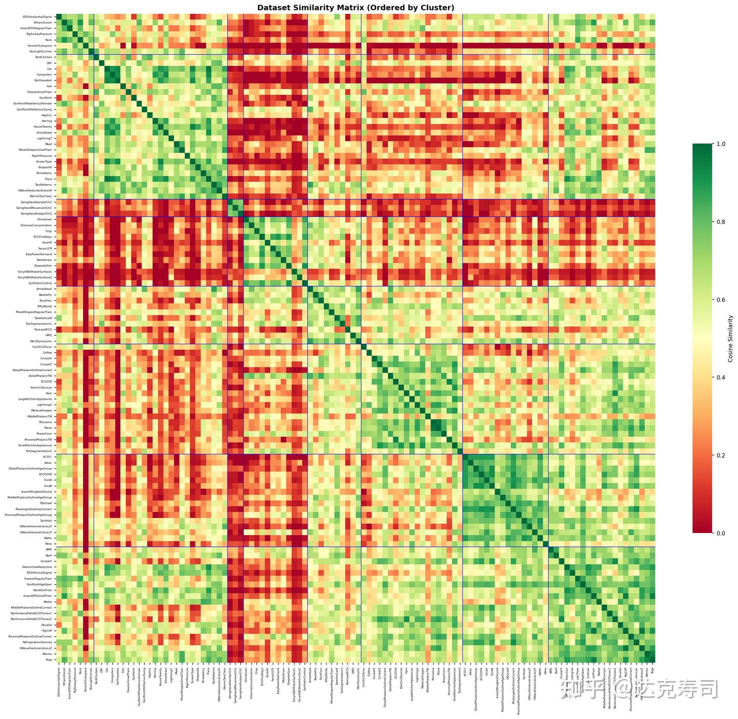
Figure 1: Correlation of wavelet evaluation metrics (UCR datasets)

In Figure 1, green indicates strong correlation and red indicates weak correlation. The matrix is partitioned into multiple blocks generated by clustering on wavelet metric values.

You can see both red and green blocks. Diagonal blocks represent clusters, where datasets tend to be more similar (greener) internally. Off-diagonal extensions show cross-cluster similarity; many of these regions are dominated by red, though some are mixed. Overall, inter-cluster correlation is relatively low, which matches the expectation that different datasets prefer different wavelet kernels. The next question is whether learned wavelet weights exhibit the same behavior.

Baseline

The baseline does not train a wavelet; it directly uses the strongest default wavelet.

Method 1: Learnable Wavelet Kernel Training

To train wavelet transforms end-to-end, we need a differentiable implementation. Common PyWavelets is not directly suitable here because its DWT is not implemented in PyTorch or TensorFlow. I implemented a differentiable DWT class in PyTorch following my earlier approach (link).

With differentiable wavelets, we can train per dataset. First, I ran a basic experiment to test whether similar data can train similar wavelet coefficients, with reconstruction-related losses. I used synthetic datasets (with explicit patterns like periodic or abrupt signals) and performed clustering on learned coefficients:

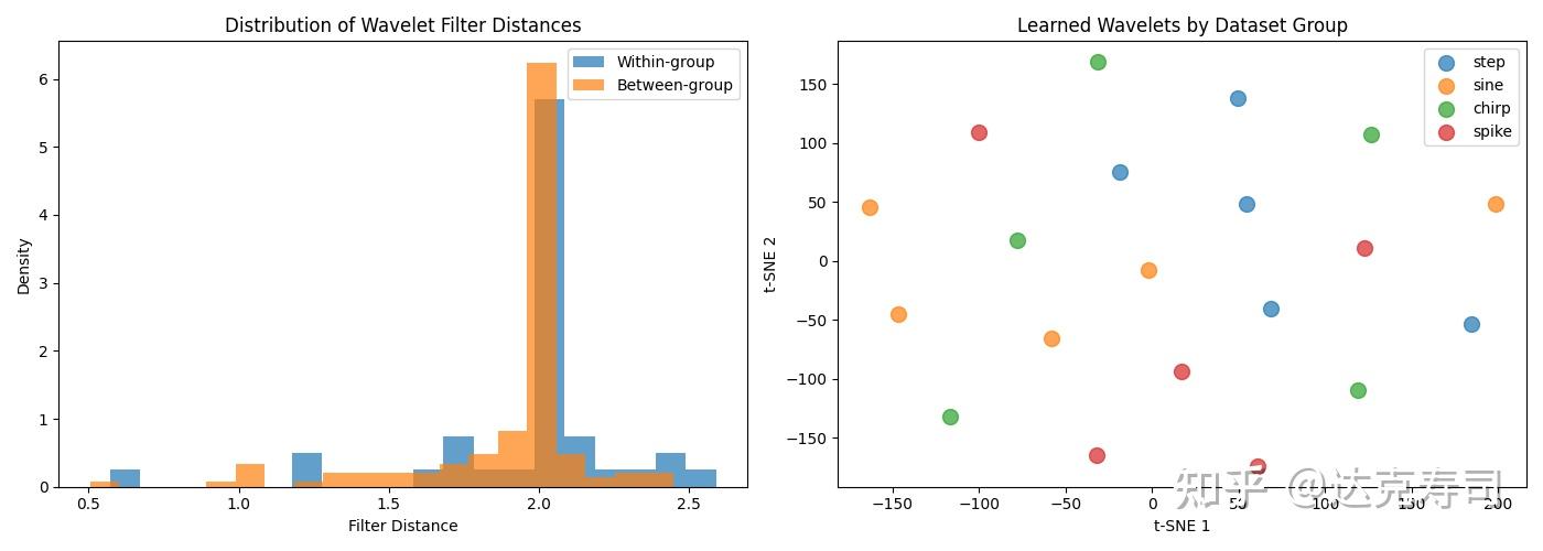
Figure 2: Inter-group vs intra-group similarity of wavelet coefficients (random initialization)

Each dataset used a learnable wavelet of length 8 with random initialization. In Figure 2 (left), intra-group and inter-group similarity distributions are almost indistinguishable. In the clustering view (right), samples from the same synthetic dataset do not cluster together. This suggests many local minima in the learnable-wavelet objective. I then repeated experiments on real UCR datasets and clustered learned coefficients with PCA and t-SNE (multiple runs per wavelet-dataset pair):

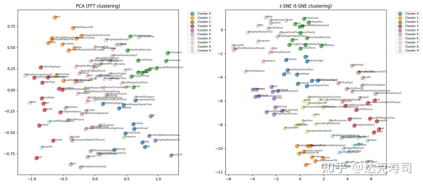
Figure 3: Clustering visualization (FFT clustering means clustering after Fourier transform of wavelet coefficients)

Many related datasets still do not cluster together, and the clustering result changes across repeated runs. So I repeated the experiment many times and plotted two example datasets:

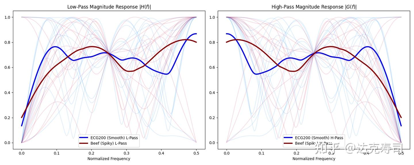
Figure 4: Results from 15 learnable-wavelet runs

All 15 runs converged to different learned kernels. Note that high-pass and low-pass filters appear mirrored because I used a QMF construction, so orthogonality is enforced by design instead of training both filters independently. Next, compare intra/inter similarity for wavelet-dataset pairs:

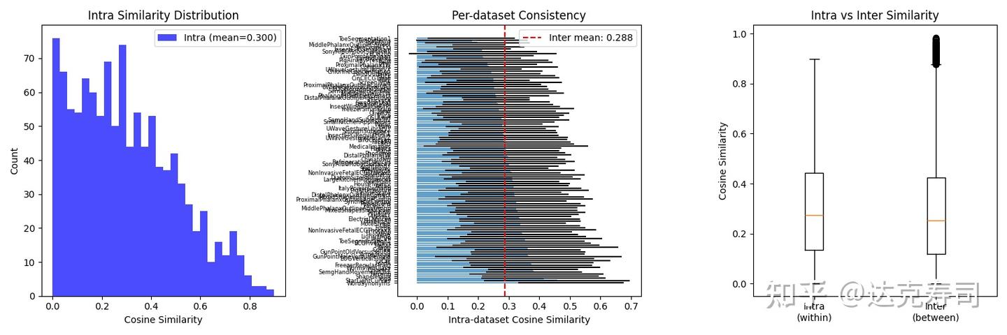
Figure 5: Intra- vs inter-similarity for wavelet-dataset pairs

Most intra-similarity values concentrate near 0 with a mean around 0.3. The box plot shows intra-similarity is only slightly higher than inter-similarity. So the hypothesis “same data produces the same learned wavelet coefficients” is not supported under random initialization. The key factor appears to be initialization. To test this, I initialized all datasets with db4 and retrained:

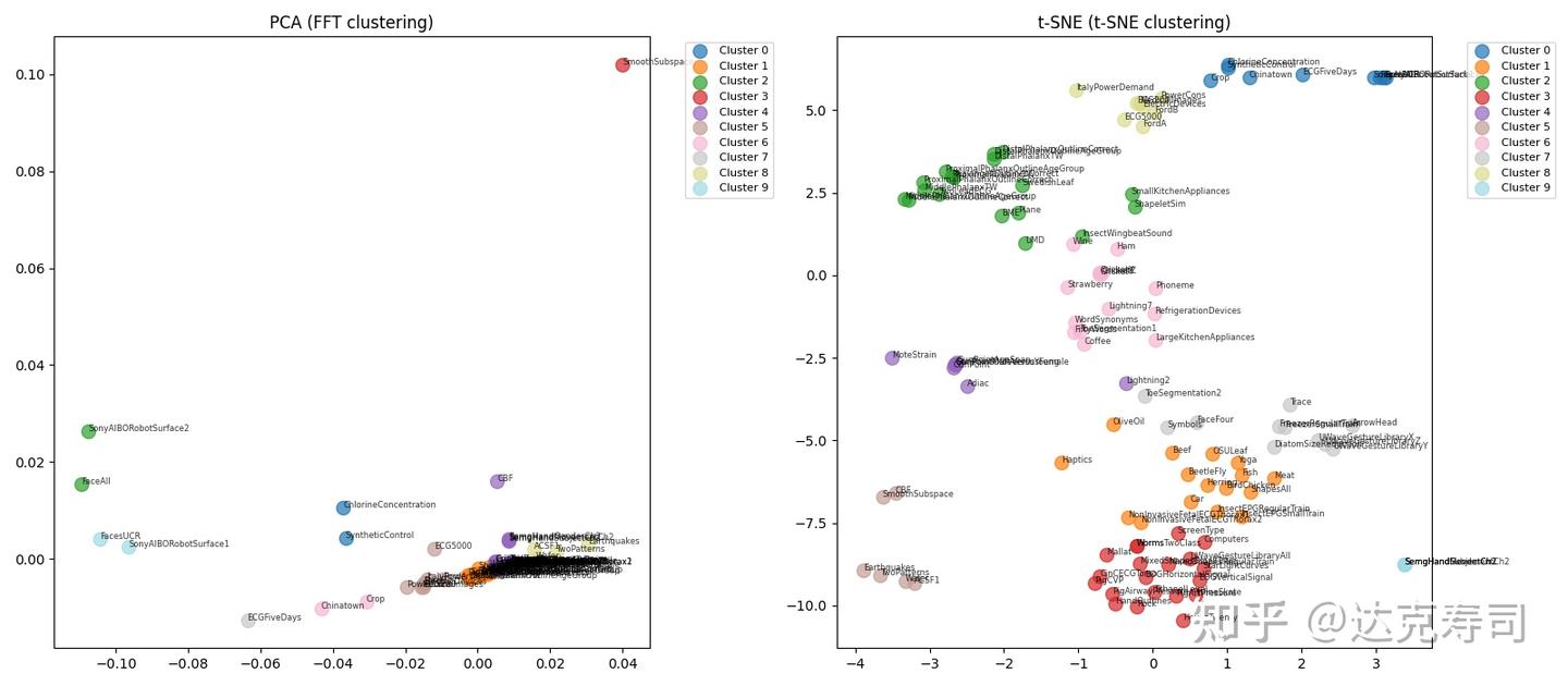
Figure 6: Clustering with db4 initialization

Now similar datasets do cluster together. Moreover, variance across 15 runs per dataset is exactly zero:

ACSF1: mean_dist=0.0000, std=0.0000
Adiac: mean_dist=0.0000, std=0.0000
ArrowHead: mean_dist=0.0000, std=0.0000
BME: mean_dist=0.0000, std=0.0000
Beef: mean_dist=0.0000, std=0.0000
BeetleFly: mean_dist=0.0000, std=0.0000
BirdChicken: mean_dist=0.0000, std=0.0000
CBF: mean_dist=0.0000, std=0.0000
......

The learned parameters are effectively identical. This means initialization almost completely determines the final solution. But in practice, this brings us back to predefined wavelets as initial weights. Another issue: all kernels here have length 8, forcing some datasets that prefer shorter wavelets to use long ones. To address this, I tried competitive learning:

models = init_model(num = n) 
for data in datasets:
    min_loss_model = get_min_loss_model(data, model) # choose the model with the minimum loss at each step
    min_loss_model.train(data)

This training strategy avoids the final clustering step, allows control over prototype count, and supports custom initial lengths per wavelet. I trained n wavelets with specified lengths and random initialization. Results (dataset names such as ACSF1, Adiac, etc.):

Training Final Assignments by Filter Length

Model	Filter Length	Datasets Assigned	Final Wins (Ep. 499)
Model 0	4	1	876
Model 1	8	83	1278
Model 2	12	1	984
Model 3	16	0	1123
Model 4	20	27	1227

Dataset Assignments

Model 0 — Length 4 (1 dataset)

ACSF1

Model 1 — Length 8 (83 datasets)

Adiac, BME, Beef, BeetleFly, CBF, Chinatown, ChlorineConcentration, Coffee, Computers, CricketX, CricketY, CricketZ, Crop, DistalPhalanxOutlineAgeGroup, DistalPhalanxOutlineCorrect, DistalPhalanxTW, ECG200, ECG5000, ECGFiveDays, Earthquakes, ElectricDevices, FaceAll, FaceFour, FacesUCR, FiftyWords, FordA, FordB, FreezerRegularTrain, FreezerSmallTrain, GunPoint, GunPointAgeSpan, GunPointMaleVersusFemale, GunPointOldVersusYoung, Ham, Haptics, HouseTwenty, InsectEPGRegularTrain, InsectEPGSmallTrain, InsectWingbeatSound, ItalyPowerDemand, LargeKitchenAppliances, Lightning2, Lightning7, Meat, MedicalImages, MiddlePhalanxOutlineAgeGroup, MiddlePhalanxOutlineCorrect, MiddlePhalanxTW, MoteStrain, NonInvasiveFetalECGThorax1, OSULeaf, OliveOil, PhalangesOutlinesCorrect, Phoneme, Plane, PowerCons, ProximalPhalanxOutlineAgeGroup, ProximalPhalanxOutlineCorrect, ProximalPhalanxTW, RefrigerationDevices, ScreenType, SmallKitchenAppliances, SonyAIBORobotSurface1, SonyAIBORobotSurface2, Strawberry, SwedishLeaf, Symbols, SyntheticControl, ToeSegmentation1, ToeSegmentation2, Trace, TwoLeadECG, TwoPatterns, UMD, UWaveGestureLibraryAll, UWaveGestureLibraryX, UWaveGestureLibraryY, UWaveGestureLibraryZ, Wafer, Wine, WordSynonyms, Worms, WormsTwoClass

Model 2 — Length 12 (1 dataset)

SmoothSubspace

Model 3 — Length 16 (0 datasets)

No datasets assigned.

Model 4 — Length 20 (27 datasets)

ArrowHead, BirdChicken, Car, CinCECGTorso, DiatomSizeReduction, EOGHorizontalSignal, EOGVerticalSignal, EthanolLevel, Fish, HandOutlines, Herring, InlineSkate, Mallat, MixedShapesRegularTrain, MixedShapesSmallTrain, NonInvasiveFetalECGThorax2, PigAirwayPressure, PigArtPressure, PigCVP, Rock, SemgHandGenderCh2, SemgHandMovementCh2, SemgHandSubjectCh2, ShapeletSim, ShapesAll, StarLightCurves, Yoga

The result is still unsatisfactory. Initialization remains a major challenge: random starts create many local minima, results vary run-to-run, and one occasionally strong wavelet dominates assignments. Most datasets choose Model 1, and some models are never selected. This could mean one strong wavelet is already sufficient, but it may still be an initialization artifact.

To mitigate this, we can initialize with predefined wavelets. Since these wavelets have strong mathematical properties, training may stay near better basins. The next problem is how to select which predefined wavelets to use. I used the globally best Top-10 wavelets from the previous post as initial prototypes; importantly, they cover diverse filter lengths:

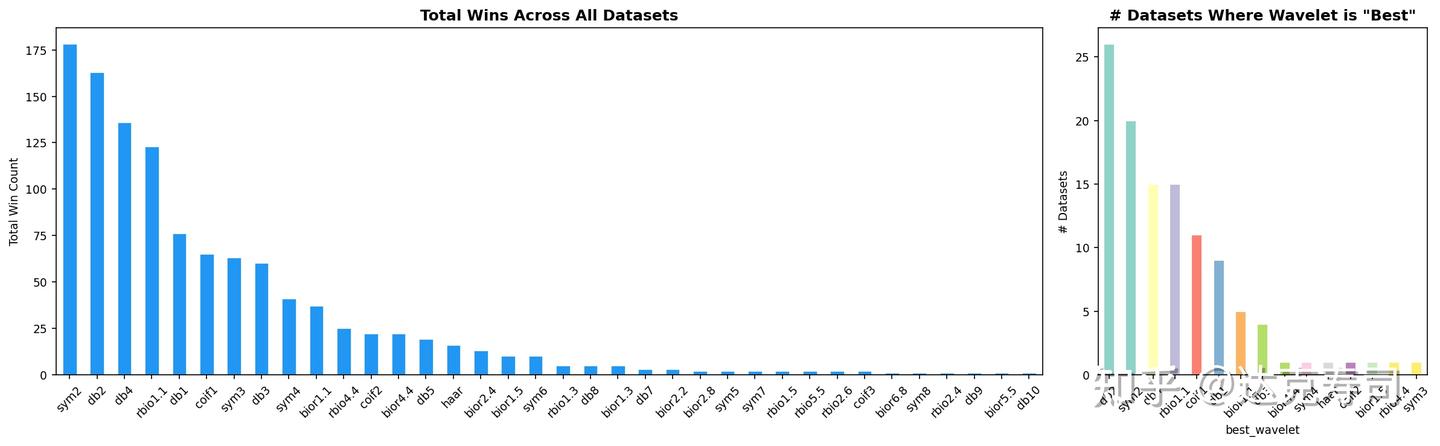
Figure 7: Strongest wavelets derived from Figure 1 (stronger if they fit more datasets)

Training results:

Final Model Assignments

Model	Filter Length	Datasets Assigned
Model 0	2	5
Model 1	34	2
Model 2	4	2
Model 3	8	0
Model 4	26	46
Model 5	32	0
Model 6	8	15
Model 7	10	16
Model 8	16	19
Model 9	10	7

Dataset Assignments

Model 0 — Length 2 (5 datasets)

Computers, Earthquakes, HouseTwenty, ScreenType, SmoothSubspace

Model 1 — Length 34 (2 datasets)

ShapeletSim, SonyAIBORobotSurface2

Model 2 — Length 4 (2 datasets)

ACSF1, Wafer

Model 3 — Length 8 (0 datasets)

No datasets assigned.

Model 4 — Length 26 (46 datasets)

BeetleFly, Car, CinCECGTorso, CricketX, CricketY, CricketZ, ECG200, ECG5000, ECGFiveDays, EOGHorizontalSignal, EOGVerticalSignal, EthanolLevel, FaceAll, FacesUCR, FordA, FordB, Ham, HandOutlines, InlineSkate, InsectEPGRegularTrain, InsectEPGSmallTrain, InsectWingbeatSound, ItalyPowerDemand, LargeKitchenAppliances, Mallat, MedicalImages, MixedShapesRegularTrain, MixedShapesSmallTrain, NonInvasiveFetalECGThorax1, NonInvasiveFetalECGThorax2, OliveOil, Phoneme, PigAirwayPressure, PigArtPressure, PigCVP, Plane, PowerCons, ProximalPhalanxOutlineAgeGroup, ProximalPhalanxOutlineCorrect, ProximalPhalanxTW, Rock, SonyAIBORobotSurface1, StarLightCurves, SwedishLeaf, Worms, WormsTwoClass

Model 5 — Length 32 (0 datasets)

No datasets assigned.

Model 6 — Length 8 (15 datasets)

Beef, CBF, Crop, Lightning2, Lightning7, Meat, MiddlePhalanxOutlineAgeGroup, MiddlePhalanxTW, MoteStrain, RefrigerationDevices, SemgHandGenderCh2, SemgHandMovementCh2, SemgHandSubjectCh2, TwoPatterns, UWaveGestureLibraryAll

Model 7 — Length 10 (16 datasets)

Chinatown, ChlorineConcentration, Coffee, DistalPhalanxOutlineAgeGroup, DistalPhalanxOutlineCorrect, DistalPhalanxTW, FaceFour, FreezerRegularTrain, FreezerSmallTrain, Haptics, MiddlePhalanxOutlineCorrect, PhalangesOutlinesCorrect, SmallKitchenAppliances, Symbols, SyntheticControl, Wine

Model 8 — Length 16 (19 datasets)

Adiac, ArrowHead, BME, BirdChicken, DiatomSizeReduction, FiftyWords, Fish, GunPoint, GunPointAgeSpan, GunPointMaleVersusFemale, GunPointOldVersusYoung, Herring, OSULeaf, ShapesAll, Strawberry, TwoLeadECG, UMD, WordSynonyms, Yoga

Model 9 — Length 10 (7 datasets)

ElectricDevices, ToeSegmentation1, ToeSegmentation2, Trace, UWaveGestureLibraryX, UWaveGestureLibraryY, UWaveGestureLibraryZ

Now, datasets assigned to each wavelet are relatively coherent. Although Model 4 (length 26) still dominates somewhat, assignments are much more balanced overall. The remaining imbalance may come from limited dataset size/diversity. Still, we have effectively compressed 106 candidate wavelets into a smaller set of prototype wavelets. Users can then pick by dataset similarity or train an ensemble directly.

Since initialization is so critical, can we train a model that predicts good initial wavelet weights for each new dataset? This leads to Method 2.

Method 2: Meta-Learning Model

If each dataset prefers different wavelets, can we learn that preference and recommend initial wavelets automatically? In [1], a method is proposed that extracts dataset meta-features and trains a regression model from meta-features to model performance. The architecture is shown below:

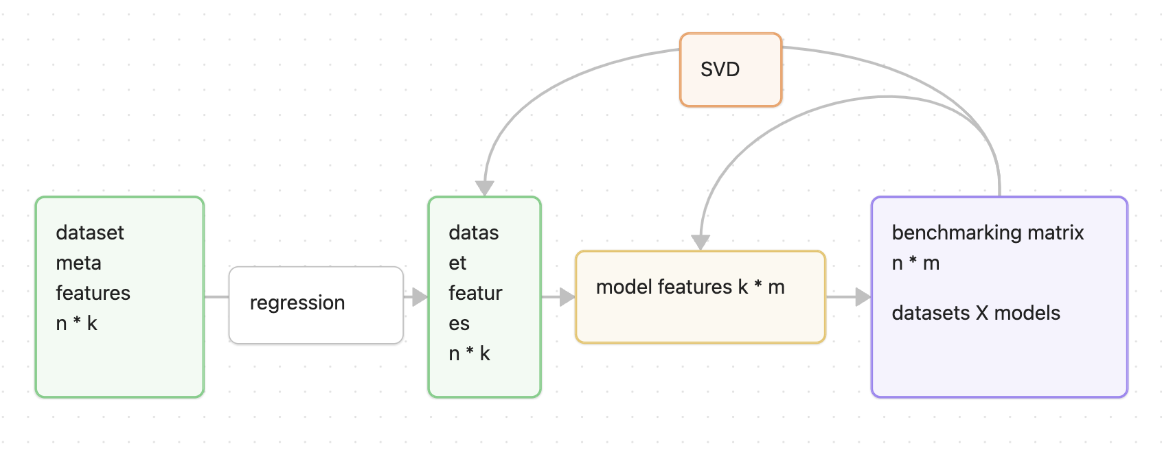
Figure 8: metaOD model architecture [1]

Originally, this method solves anomaly-detector selection: train many models on many datasets, then form a model-performance matrix. That matrix can be directly replaced by our dataset-wavelet matrix. The only trainable component is a multi-output regressor mapping dataset meta-features to latent dataset embeddings (metaOD [1] uses random forest). Meta-features can be handcrafted (descriptive stats, frequency-domain features, etc.). In [2], TabPFN provides a strong zero-shot model for tabular features; we can also use its embeddings by flattening time steps.

After training the regressor, we can recommend wavelets for unseen datasets:

$1k_{new-meta} = f(1k_{new})$, where $f$ is the random-forest regressor

$performance(1m) = 1k_{new-meta} * k*m$

This performance vector is the predicted wavelet performance. It is fast, and allows model selection before full training. Absolute values are less important than ranking. We evaluate quality by Top-5 coverage. To test whether the model captures data-performance relationships, I evaluated separate/combined UCR and LOTSA settings, and also TabPFN embeddings as meta-features (baseline: choose benchmark Top-10 wavelets directly):

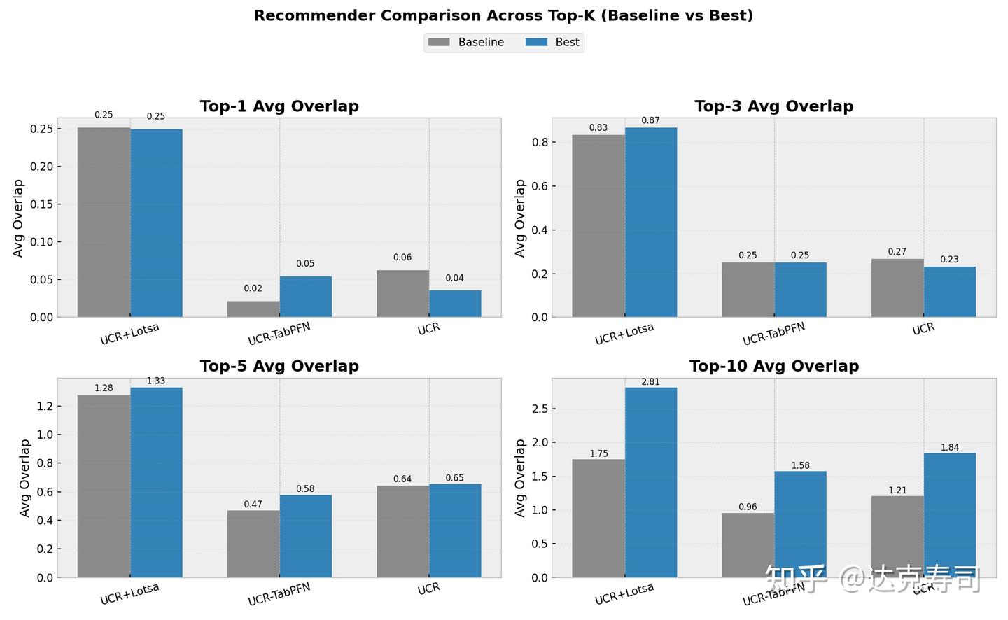
Figure 9: metaOD model results

The axes represent overlap between recommended models and the true Top-K models. We care about overlap, not exact rank order; different models correspond to different wavelets. Results are often better than baseline, but even for Top-5 the model typically recovers only around one correct wavelet on average. For Top-10 recommendation, larger dataset collections seem to help. TabPFN meta-features appear better than my handcrafted features. Overall, this is still not ideal. (In the figure, UCR_TabPFN uses a different baseline than UCR because TabPFN cannot handle some large-sample datasets, so those were removed.)

I then proposed a new model: a CNN meta-learner. The bottleneck seems to be the number of datasets. Getting many diverse new time-series datasets is difficult because each new dataset also requires full wavelet-performance profiling. So instead of dataset-level training, I switched to sample-level training: each sample maps to the performance distribution of its source dataset. This greatly increases training data, since each dataset has at least ~50 samples. For time series, a single sequence can itself be treated as a dataset; windowed/sliding samples naturally support this view.

Model architecture:

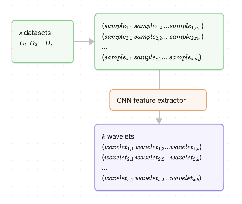
Figure 10: CNN meta-learning architecture

The model maps samples in a dataset (sample1..n) directly to the wavelet performance vector (wavelet1..k) for that dataset, reducing overfitting risk by increasing training instances. The training objective uses a rank loss [3]:

$$ \Delta_{b,i,j} = \hat{y}_{b,i} - \hat{y}_{b,j} $$

Here $\Delta_{b,i,j}$ is the predicted score difference between a true Top-5 item and a non-Top-5 item for sample $b$. Then apply softplus:

$\ell_{b,i,j} = \log(1 + e^{\Delta_{b,i,j}})$

Final rank loss:

$\mathcal{L}_{\text{rank}} = \frac{1}{|T_b| \times |N_b|}\sum \ell$

A simple example:

Computation rule: $\Delta_{b,i,j} = \hat{y}_i - \hat{y}_j$

All $(i,j)$ pairs with $i \in T_b$ and $j \in N_b$, where $T_b$ is the true Top-K set (good items) and $N_b$ is the non-Top-K set (bad items):

Consider one sample $b=1$ and 5 wavelets (indices 0-4).

True score $y$ (from CSV)

y = [0.1, 0.8, 0.9, 0.2, 0.7]
     w0   w1   w2   w3   w4

Model prediction $\hat{y}$ (current scores)

ŷ = [0.15, 0.7, 0.85, 0.3, 0.6]
     w0    w1    w2    w3    w4

Step 1: Define Top-2 using true $y$

Sort by true scores:

w2(0.9) > w1(0.8) > w4(0.7) > w3(0.2) > w0(0.1)

So:

Top-2 set:    T_b = {w2, w1}  (should be in Top-2)
Other set:    N_b = {w0, w3, w4}  (should not be in Top-2)

Pair	Positive item i	Negative item j	Pred(i)	Pred(j)	Delta = Pred(i) - Pred(j)
1	w2	w0	0.85	0.15	0.70
2	w2	w3	0.85	0.30	0.55
3	w2	w4	0.85	0.60	0.25
4	w1	w0	0.70	0.15	0.55
5	w1	w3	0.70	0.30	0.40
6	w1	w4	0.70	0.60	0.10

Step 3: Softplus penalty

Formula:

$\ell_{b,i,j} = \log(1 + e^{\Delta_{b,i,j}})$

Pair	Delta	e^Delta	1+e^Delta	loss_b,i,j
1	0.70	2.01	3.01	1.10
2	0.55	1.73	2.73	1.00
3	0.25	1.28	2.28	0.82
4	0.55	1.73	2.73	1.00
5	0.40	1.49	2.49	0.91
6	0.10	1.11	2.11	0.74

Step 4: Compute rank loss

Formula:

$\mathcal{L}_{\text{rank}} = \frac{1}{|T_b| \times |N_b|}\sum \ell$

Computation:

$\mathcal{L}_{\text{rank}} = \frac{1}{2 \times 3}(1.10 + 1.00 + 0.82 + 1.00 + 0.91 + 0.74)$

$= \frac{5.57}{6} = 0.928$

Training result:

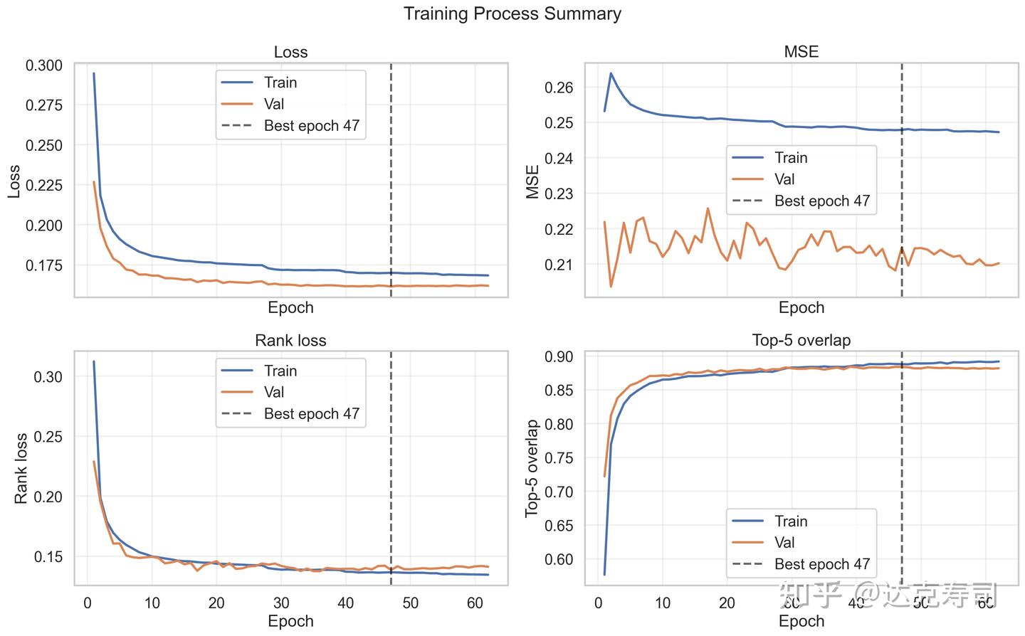
Figure 11: Model training process

MSE does not change much, but Top-5 coverage steadily increases during training. This is exactly what we need: score calibration is less important than ranking quality. Next, we inspect whether the model relies on trivial predictions (i.e., giving almost the same output for every dataset):

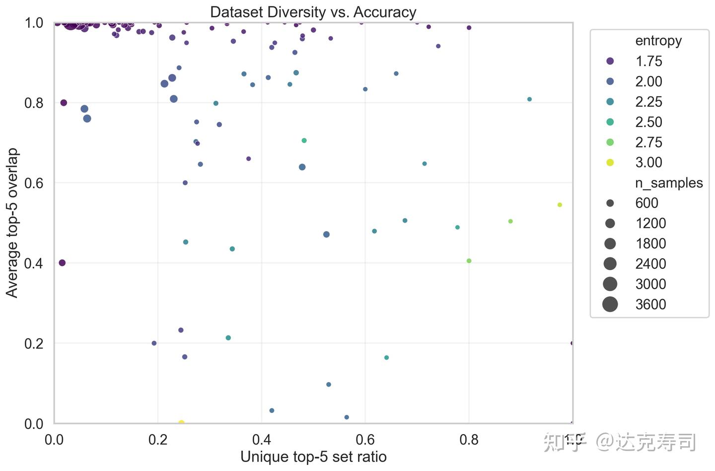
Figure 12: Data diversity vs Top-5 prediction accuracy

From the figure, many high-accuracy predictions (upper-left area) have relatively low diversity. If we relax accuracy, diversity increases. This suggests the model provides personalized predictions in roughly half the cases. But this could also be caused by low diversity in the original labels (wavelet scores). So we inspect label diversity next:

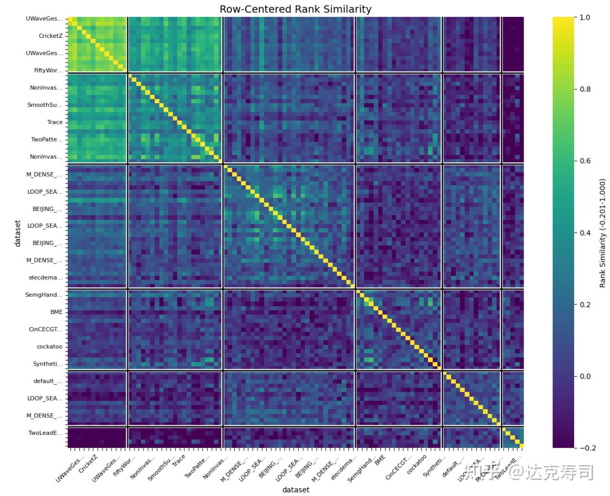
Figure 13: Centered-rank similarity of wavelet performance across datasets

Compared with Figure 1, diversity in true wavelet performance is lower than diversity in metric values, but diversity still clearly exists. This supports that the model’s ~88% accuracy is not merely from trivial prediction. Therefore, the meta-learning model is reasonably reliable. For a new dataset with multiple time-series samples, we can perform zero-shot prediction per sample, vote for the top-5 wavelets, use them as initialization candidates, and then train learnable wavelets for downstream tasks.

Finally, does a learnable wavelet actually outperform predefined wavelets? I ran the following experiments:

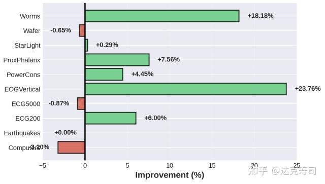
Figure 14: With wavelet transform vs without wavelet transform

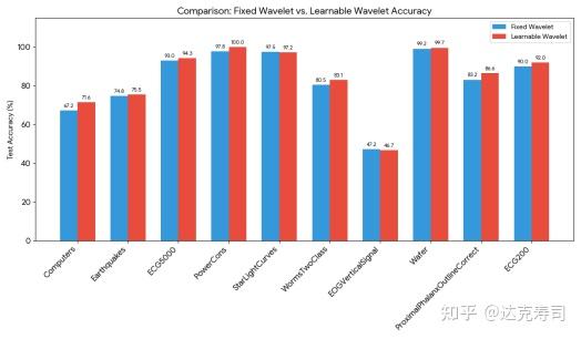
Figure 15: Fixed wavelet parameters (db4) vs learnable wavelet

To reduce confounding factors, I first checked whether wavelet transforms help time-series classification at all. Figure 14 shows that in most cases they help significantly, and when they do not help, they usually do not hurt much. Figure 15 shows that learnable wavelets generally outperform fixed db4, so they are beneficial for downstream tasks, though gains are often modest.

This likely concludes my wavelet-transform series. After many experiments, my takeaway is that wavelet transforms are a useful but relatively small component in machine learning systems. Their strengths appear most clearly when integrated with other models in practical engineering pipelines. In my experiments, adding wavelet transform was not always essential, though this may also reflect limitations in my own engineering experience. Feedback is very welcome.

Appendix

References

[1] Yue Zhao, Ryan A. Rossi, Leman Akoglu. “Automating Outlier Detection via Meta-Learning”. arXiv:2009.10606 [cs.LG]. https://doi.org/10.48550/arXiv.2009.10606

[2]Noah Hollmann, Samuel Müller, Katharina Eggensperger, Frank Hutter. “TabPFN: A Transformer That Solves Small Tabular Classification Problems in a Second”. arXiv:2207.02045 [cs.LG]. https://doi.org/10.48550/arXiv.2207.02045

[3]Rendle, S., Freudenthaler, C., Gantner, Z., & Schmidt-Thieme, L. (2012). BPR: Bayesian Personalized Ranking from Implicit Feedback. arXiv:1205.2618 [http://cs.IR]. https://doi.org/10.48550/arXiv.1205.2618