In the last essay we talked about using the Gamma-Poisson conjugate distribution to develop trading strategies. In the following article, we will try to use the more complex Dirichlet-Multinominal conjugate distribution.
What is Dirichlet Distribution
The Dirichlet distribution is a family of continuous multivariate probability distributions parameterized by a positive real vector. It is often used as a prior distribution for multinomial distributions in Bayesian statistics. The formula for the probability density function of the Dirichlet distribution is as follows:
$$ P(\mathbf{x} \mid \boldsymbol{\alpha}) = \frac{1}{B(\boldsymbol{\alpha})} \prod_{i=1}^{K} x_i^{\alpha_i - 1} $$where $\mathbf{x} = (x_1, \ldots, x_K)$ is a K-dimensional vector representing the probabilities of K different categories or events. The sum of these probabilities must be 1.
$\boldsymbol{\alpha} = (\alpha_1, \ldots, \alpha_K)$ is a positive parameter vector, $\alpha_i$ represents the prior, or count, of the $i$th category.
$\beta(\alpha)$ is the polynomial Beta function, which serves as a normalization constant to ensure that the total probability integral is 1. It is defined as: $B(\boldsymbol{\alpha}) = \frac{\prod_{i=1}^{K} \Gamma(\alpha_i)}{\Gamma\left(\sum_{i=1}^{K} \alpha_i\right)}$, where $\Gamma$ represents the Gamma function, which is an extension of the factorial function (whose argument is shifted down by 1) to real and complex numbers.
The Dirichlet distribution is a generalization of the Beta distribution to higher dimensions. In the two-dimensional case (K=2), the Dirichlet distribution simplifies to the Beta distribution.
What is Multinomial distribution?
The multinomial distribution is a generalization of the binomial distribution to more than two categories. It describes the probability of each possible count for rolling a K-sided die n times. In simple terms, it is the distribution of the counts of multiple categories in a fixed number of trials.
Features:
- Class: There are K possible outcomes or classes.
- Trial: There are n independent trials.
- Probability: Each trial produces exactly one of the K classes. The probability of each class in each trial is fixed and expressed as: $p_1,p_2,\dots,p_k$, where $∑p_i=1$
Probability Mass Function(PMF): The pmf of the multinomial distribution of a given outcome $x=(x_1,x_2,\dots,x_K)$ is:
$$P(X = x) = \frac{n!}{x_1! x_2! \ldots x_K!} p_1^{x_1} p_2^{x_2} \ldots p_K^{x_K} $$Where $x_i$ is the count of the $i$ category, and $\sum_{i=1}^{K} x_{i} = n$.
Conjugate Prior
In Bayesian statistics, a conjugate prior is a prior distribution that, when combined with a likelihood function, produces a posterior distribution of the same family. For multinomial distributions, the conjugate prior is the Dirichlet distribution.
Principle: Prior: Before observing any data, we express our belief about the class probabilities using a Dirichlet distribution (characterized by parameters) with parameters $\boldsymbol{\alpha} = (\alpha_1,\alpha_2, \ldots, \alpha_K)$ Likelihood: Then we observe data which can be modeled as a multinomial distribution. Posterior: After observing the data, the posterior distribution of the class probabilities is again a Dirichlet distribution but with updated parameters.
Update parameters: The parameters of the Dirichlet prior are updated in a simple way based on the observed data. If the original parameters are $\boldsymbol{\alpha} = (\alpha_1,\alpha_2, \ldots, \alpha_K)$, and the observed counts are $x=(x_1,x_2,\dots,x_K)$, the parameters of the Dirichlet posterior distribution are: $\boldsymbol{\alpha} + x = (\alpha_1+x_1,\alpha_2+x_2, \ldots, \alpha_K+x_K)$
The concept of a conjugate prior, such as the Dirichlet-multinomial, is crucial in Bayesian analysis because it simplifies the computation of the posterior distribution, which is the basis of Bayesian inference. This conjugation allows for more straightforward analysis or computational updates to our beliefs in light of new data.
Tips
- The meaning of parameter $\alpha_i$:
- When $\alpha_i$ is greater than 1, it indicates that the corresponding category $i$ has a higher prior probability.
- When $\alpha_i$ is equal to 1, it indicates that there is no special prior knowledge about these categories, which is called uninformative prior.
- When $\alpha_i$ is less than 1, it indicates that the corresponding category $i$ has a lower prior probability.
- Expression of probability:
- In the Dirichlet distribution, the expected value of $p_i$ (the probability of the $i$th category) is $E[p_i]=\frac{\alpha_{i} }{\sum_{j=1}^{k} \alpha_{j} }$ . This shows that $\alpha_i$ affects the probability of the corresponding category, but is not directly equivalent to the probability.
- Bayesian Update:
- After the data is observed, the parameters of the Dirichlet distribution are updated to form the posterior distribution. If the number of times category $i$ appears in the observed data is $x_i$, then the parameters of the posterior distribution become $\alpha_i+x_i$. This means that each $\alpha_i$ as prior knowledge combined with the observed data jointly affects the posterior probability of category $i$. Therefore, each $\alpha_i$ can be regarded as a “belief” or expectation of the probability of category $i$ before the data is observed, and these beliefs are updated as the data appears. This is a core feature of the Bayesian method: combining prior beliefs and observed data to form posterior knowledge.
Parameter Update Visualization
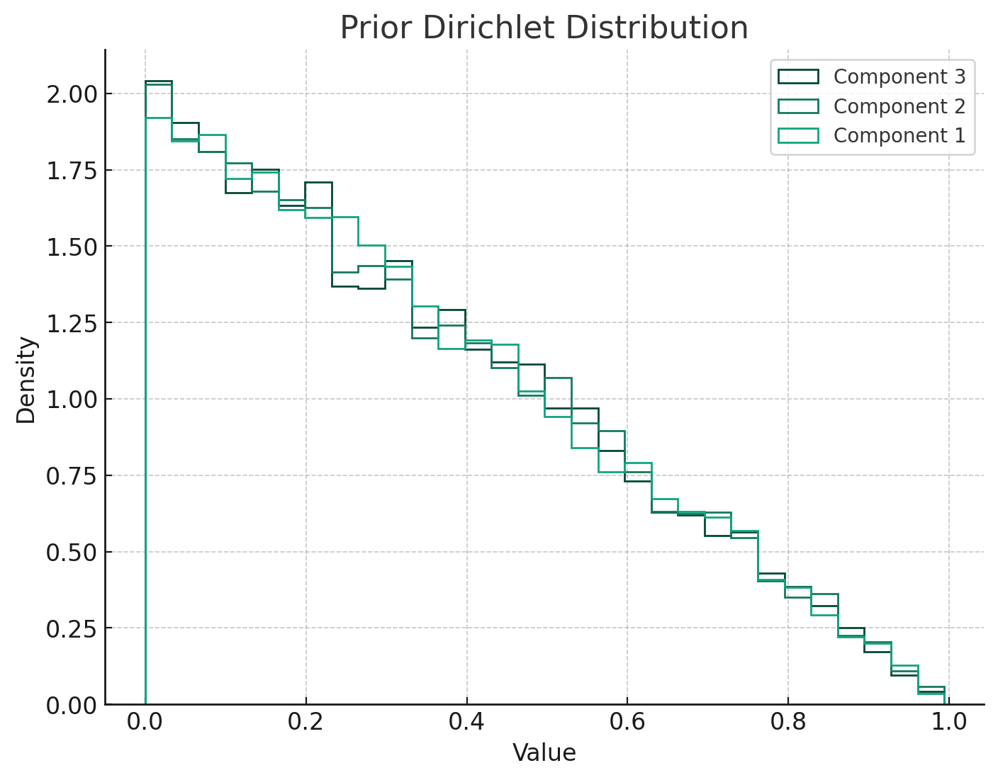
- Prior Dirichlet Distribution: This distribution represents our initial beliefs about the probabilities of different outcomes (in the 3-class example). Here, I used a uniform prior with parameters [1,1,1], indicating no initial preference for any class.
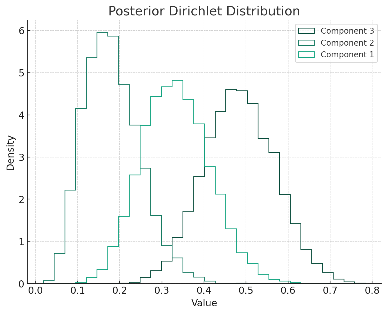
- Posterior Dirichlet Distribution: After observing the data (in this case, [10,5,15] counts for each class), the posterior distribution updates our beliefs. The parameters of the posterior distribution are the sum of the prior parameters and the observed counts, resulting in parameters [11,6,16]. This posterior distribution now reflects our updated beliefs after taking into account the observed data.
import numpy as np
import matplotlib.pyplot as plt
from scipy.stats import dirichlet

# Function to plot Dirichlet distributions
def plot_dirichlet(parameters, title):
    # Sample from the Dirichlet distribution
    samples = dirichlet.rvs(parameters, size=10000)

    # Plotting
    plt.figure(figsize=(8, 6))
    plt.hist(samples, bins=30, density=True, histtype='step', label=['Component 1', 'Component 2', 'Component 3'])
    plt.title(title)
    plt.xlabel('Value')
    plt.ylabel('Density')
    plt.legend()
    plt.show()

# Prior Dirichlet distribution parameters (example values)
prior_parameters = np.array([1, 1, 1])
plot_dirichlet(prior_parameters, "Prior Dirichlet Distribution")

# Dirichlet-multinomial conjugation: updating the parameters
# Let's say we have observed counts for each category
observed_counts = np.array([10, 5, 15]) # example counts for 3 categories
posterior_parameters = prior_parameters + observed_counts
plot_dirichlet(posterior_parameters, "Posterior Dirichlet Distribution")
Trading strategy
In this strategy, you use long-term data to set the prior parameters, and then use short-term data to update the posterior parameters to make trading decisions. Here is one way to implement this strategy:
Step 1: Set Prior Parameters
- Choose Long-Term Data: First, you need to decide what kind of data represents the long-term. For example, this could be monthly data for the past year, or any other historical data that fits your strategy.
- Analyze Long-Term Data: Based on this data, you can estimate the frequency of each category (e.g., “bullish”, “bearish”, “neutral”).
- Set Dirichlet Prior Parameters: Use these frequencies to set the prior parameters of the Dirichlet distribution $\boldsymbol{\alpha} = (\alpha_1,\alpha_2, \ldots, \alpha_K)$, which reflect your initial beliefs about the long-term market behavior.
    def on_long_bar(self, long_bar: BarData):
        self.am_long.update_bar(long_bar)
        if not self.am_long.inited:
            return

        # Calculate the number of bullish, bearish and neutral bars
        for i in range(self.am_long.size):
            diff = self.am_long.close[i] - self.am_long.open[i]
            tick_diff = diff/self.tick_size
            if tick_diff > self.tick_size_threshold:
                self.prior_bullish += 1
            elif tick_diff < -self.tick_size_threshold:
                self.prior_bearish += 1
            else:
                self.prior_neutral += 1

        self.prior_neutral = self.prior_neutral/self.am_long.size
        self.prior_bearish = self.prior_bearish/self.am_long.size
        self.prior_bullish = self.prior_bullish/self.am_long.size

        self.priors_inited = True
Step 2: Update the posterior parameters
- Select short-term data: Next, select data that represents a short period, such as the data from the last week or month.
- Calculate category counts: Count the number of occurrences of each category in the short period.
- Update the posterior parameters: Use the short-term data to update the prior parameters. If the category counts you observe in the short period are $(x_1,x_2,\dots,x_k)$, then the posterior parameters are $\boldsymbol{\alpha_{post}} + x = (\alpha_1+x_1,\alpha_2+x_2, \ldots, \alpha_K+x_K)$
    def on_short_bar(self, short_bar: BarData):
        self.am_short.update_bar(short_bar)
        if not self.am_short.inited:
            return

        if not self.priors_inited:
            return

        buy_signal = False
        sell_signal = False

        bullish_count = 0
        bearish_count = 0
        neutral_count = 0

        # Calculate the number of bullish, bearish and neutral bars
        for i in range(self.am_short.size):
            diff = self.am_short.close[i] - self.am_short.open[i]
            tick_diff = diff/self.tick_size
            if tick_diff > self.tick_size_threshold:
                bullish_count += 1
            elif tick_diff < -self.tick_size_threshold:
                bearish_count += 1
            else:
                neutral_count += 1

        # Parameter updating
        self.post_bullish = self.prior_bullish + bullish_count
        self.post_bearish = self.prior_bearish + bearish_count
        self.post_neutral = self.prior_neutral + neutral_count
Step 3: Make a trading decision
- Calculate the posterior mean: Calculate the posterior probability of each class, $\alpha_{j\text{post}} = \frac{\alpha_{j\text{post}}}{\sum_{i=1}^{k} a_{i\text{post}}}$
- Select the class with the highest probability: Based on the posterior mean, determine which class has the highest probability.
- Develop a trading strategy: Develop your trading strategy based on the class with the highest probability. For example, if the “bullish” class has the highest probability, you might choose to buy; if it is “bearish”, you might choose to sell.
sumpost = self.post_bearish+self.post_neutral+self.post_bullish

        post_prob_bull = self.post_bullish/sumpost
        post_prob_bear = self.post_bearish/sumpost
        post_prob_neu = self.post_neutral/sumpost


        maxValue = max(post_prob_neu,post_prob_bull,post_prob_bear)

        if maxValue == post_prob_bear:
            sell_signal = True
        elif maxValue == post_prob_bull:
            buy_signal = True
        else:
            return

        if self.dual_side:
            if buy_signal and sell_signal:
                return
            # both long and short
            if buy_signal:
                if self.pos >= 0:
                    if abs(self.pos) < self.pyramiding:
                        self.buy(short_bar.close_price, self.fix_size)
                else:
                    self.cover(short_bar.close_price, abs(self.pos))
                    self.buy(short_bar.close_price, self.fix_size)

            if sell_signal:
                if self.pos <= 0:
                    if abs(self.pos) < self.pyramiding:
                        self.short(short_bar.close_price, self.fix_size)
                else:
                    self.sell(short_bar.close_price, abs(self.pos))
                    self.short(short_bar.close_price, self.fix_size)

        else:
            if buy_signal:
                if self.pos >= 0 and self.pos < self.pyramiding:
                    self.buy(short_bar.close_price, self.fix_size)

            if sell_signal:
                if self.pos != 0:
                    self.sell(short_bar.close_price, self.pos)
Strategy Practice
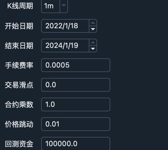
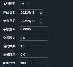
Environment parameter
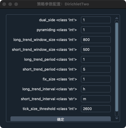
 Strategy parameter
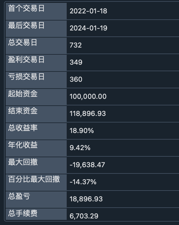
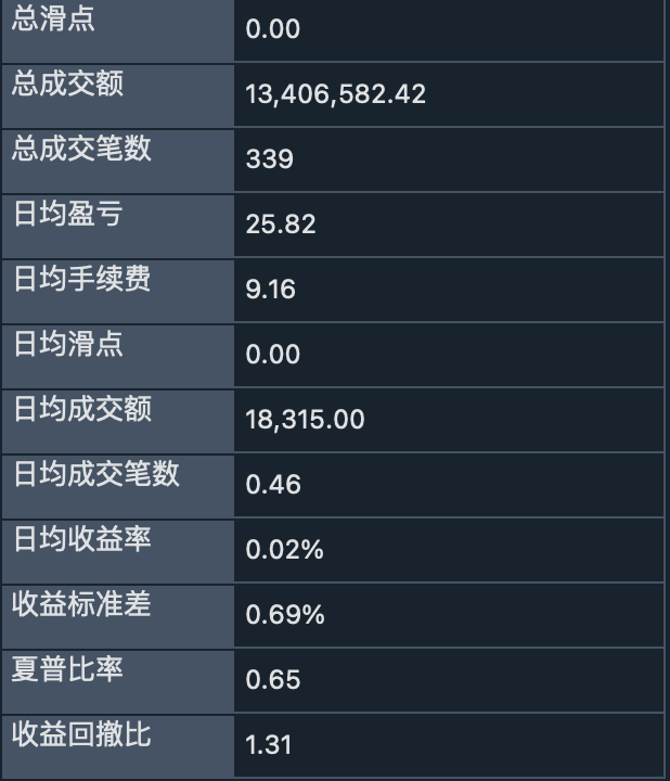
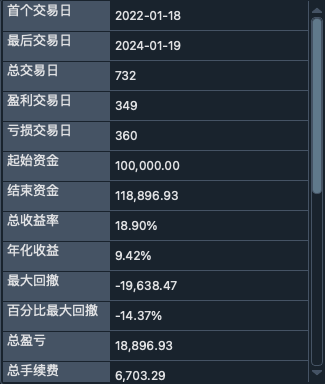
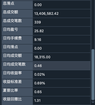
 backtesting result
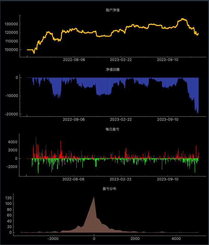
 Strategy curve