In the previous post we learned how to design trading strategies using the beta-binomial conjugate distribution. Can we design trading strategies using the gamma-Poisson conjugate distribution? This post will show an example of a trading strategy.
Model
- Objective: simulate the average number of increases over a period of time
- Prior distribution: gamma distribution, the following is the distribution function of gamma distribution:
Below are the images of the gamma distribution function with different parameters::
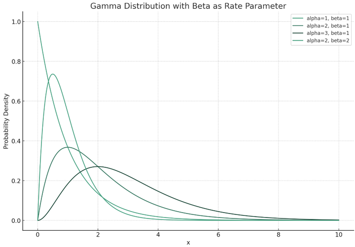 It can be seen that the domain of the gamma distribution is [0, +$\infty$], which means that we can no longer choose to study the parameter $\theta$, which is a 0 to 1 probability of increase. We can study the average number of increases $\lambda$ over a period of time. This is why we need to choose the Poisson distribution to calculate the likelihood.
- Poisson distribution likelihood function:
Poisson distribution has only one parameter $\lambda$, which we define as the number of increases in a period of time.
The following is the probability density function of Poisson distribution:
$$L(\lambda; k) = \frac{e^{-\lambda} \lambda^k}{k!}$$
The following is the probability density image of Poisson distribution:
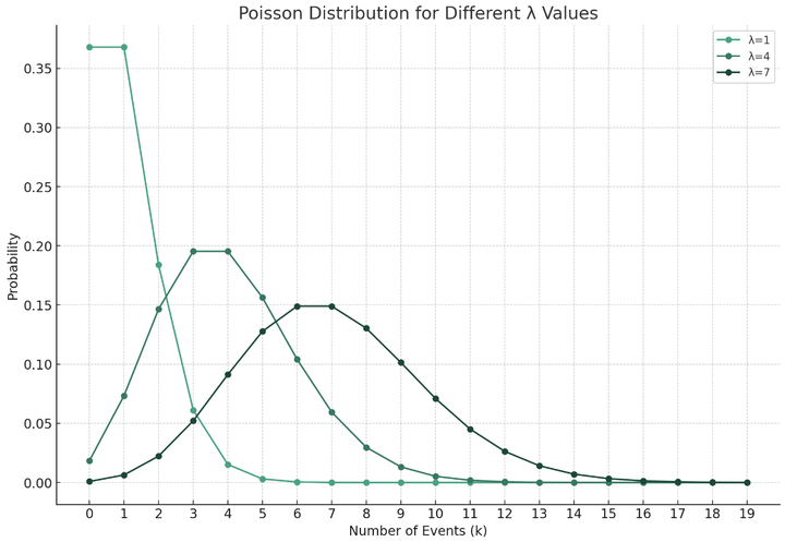 It can be seen that the Poisson distribution is a discrete distribution, which can be used to simulate discrete values such as the number of increases.
If we assume that the number of increases in each period of time is independent of each other, we can use the Poisson likelihood function.
The following is the likelihood function of the Poisson distribution:
$$L(\lambda; x_1, x_2, \ldots, x_n) = e^{-n\lambda} \lambda^{\sum_{i=1}^{n}x_i} \prod_{i=1}^{n} \frac{1}{x_i!} $$
It can be seen that the Poisson distribution is a discrete distribution, which can be used to simulate discrete values such as the number of increases.
If we assume that the number of increases in each period of time is independent of each other, we can use the Poisson likelihood function.
The following is the likelihood function of the Poisson distribution:
$$L(\lambda; x_1, x_2, \ldots, x_n) = e^{-n\lambda} \lambda^{\sum_{i=1}^{n}x_i} \prod_{i=1}^{n} \frac{1}{x_i!} $$ - Posterior distribution After we have the prior distribution and likelihood function, we can calculate the posterior distribution, which is as follows: $$p(\lambda | x_1, x_2, \ldots, x_n; \alpha', \beta') = \frac{{\beta'}^{\alpha'}}{\Gamma(\alpha')} \lambda^{\alpha' - 1} e^{-\beta' \lambda} $$ $$\alpha' = \alpha + \sum_{i=1}^{n} x_i,\beta' = \beta + n$$ It can be found that the posterior distribution is also a gamma distribution, and the $\alpha$ and $\beta$ of the posterior distribution can be directly obtained through the information of the observed samples, which provides great convenience for the calculation.
Application Examples
-
Long cycle The long cycle determines the gamma distribution prior. The unit of the long cycle is hour k. The long cycle sequence is hour k of n days, which is synthesized by 7 * 24 * 60 = 10080 minute k. Then calculate the number of daily increases in 24 hours, {“day1”: 13, “day2”: 6, “day3”: 8….“dayn”: x} Calculate the sample mean and variance to estimate (Moment method, moment estimation) the prior alpha prior and beta prior $\bar{x} = \frac{\alpha}{\beta}$,$s^2 = \frac{\alpha}{\beta^2}$
-
Short cycle The short cycle determines the likelihood function. The unit of the short cycle is minute k. The length of the number cycle n may not be equal to that of the long cycle. The range of the number of short-term rises should preferably include the range of the number of long-term rises, that is, $\lambda_{long} \subseteq \lambda_{short}$, because if the maximum number of short-term rises is 3 and the maximum number of long-term rises is 12, the posterior probability distribution will definitely move toward a smaller $\lambda$ value, which will cause us to lose some information. So we assume that the maximum number of rises per cycle in such a short cycle is 24, that is, I need n 24 minute k, a total of n * 24 minute K lines. Get the short-term data {“k1”: 13, “k2”: 12, “k3”:9 , …..“kn”:x}
Code simulation and implementation
First, I randomly select 50 samples according to the number of increases range [0,24], and then calculate the mean and variance of this sample.
long_period_data = np.random.randint(0, 25, 50)  # 假设每天的最大上涨次数为24

# Calculate mean and variance
mean_long = np.mean(long_period_data)
variance_long = np.var(long_period_data)

# Estimate prior parameters of the gamma distribution
alpha_prior = mean_long**2 / variance_long
beta_prior = mean_long / variance_long
Finally, the prior $\alpha$ and $\beta$ values are calculated using moment estimation. The next step is to simulate short-term data, also using random function sampling.
#Simulate short-term (24-minute) data
    short_period_data = np.random.randint(0, 25, size=5)  # 假设每24分钟周期的最大上涨次数为24

# Update the posterior distribution parameters
    alpha_posterior = alpha_prior + sum(short_period_data)
    beta_posterior = beta_prior + len(short_period_data)
Finally, the posterior parameters are calculated according to the formula of the conjugate posterior distribution mentioned above.
The following is an image comparison:
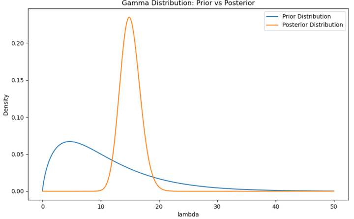 It can be seen that the mean and mode of the posterior distribution have moved to the right, indicating that the average number of increases observed in the short period may be relatively high, causing the distribution to move to the right.
Comparison of prior and posterior parameters:
It can be seen that the mean and mode of the posterior distribution have moved to the right, indicating that the average number of increases observed in the short period may be relatively high, causing the distribution to move to the right.
Comparison of prior and posterior parameters:
Alpha Prior: 1.7518570171605738, Beta Prior: 0.16190915130874067
Alpha Posterior: 77.75185701716057, Beta Posterior: 5.16190915130874
Case complete code:
import numpy as np
from scipy.stats import gamma, poisson
import matplotlib.pyplot as plt
for i in range(5):
    #Simulate long-term data
    long_period_data = np.random.randint(0, 25, 50) # Assume that the maximum number of daily increases is 24

   # Calculate mean and variance
    mean_long = np.mean(long_period_data)
    variance_long = np.var(long_period_data)

    # Estimate the prior parameters of the gamma distribution
    alpha_prior = mean_long**2 / variance_long
    beta_prior = mean_long / variance_long

   #Simulate short-term data
    short_period_data = np.random.randint(0, 25, size=5)  # Assume that the maximum number of increases per 24-minute period is 24

    # Update the posterior distribution parameters
    alpha_posterior = alpha_prior + sum(short_period_data)
    beta_posterior = beta_prior + len(short_period_data)

    # Output results
    print(f"Alpha Prior: {alpha_prior}, Beta Prior: {beta_prior}")
    print(f"Alpha Posterior: {alpha_posterior}, Beta Posterior: {beta_posterior}")

    # Create prior and posterior distributions for the gamma distribution
    prior_dist = gamma(alpha_prior, scale = 1/beta_prior)
    posterior_dist = gamma(alpha_posterior, scale = 1/beta_posterior)
    lambda_samples = np.random.gamma(alpha_posterior, 1/beta_posterior, 1000)

    # Generate gamma distribution probability density function (PDF) data
    x = np.linspace(0, 50, 100000)
    y_prior = prior_dist.pdf(x)
    y_posterior = posterior_dist.pdf(x)

    # Draw the image
    plt.figure(figsize=(10, 6))
    plt.plot(x, y_prior, label='Prior Distribution')
    plt.plot(x, y_posterior, label='Posterior Distribution')
    plt.title('Gamma Distribution: Prior vs Posterior')
    plt.xlabel('lambda')
    plt.ylabel('Density')
    plt.legend()
    plt.show()
Strategy Backtesting
Strategy Logic
Logic 1: After obtaining the parameters of the posterior distribution, calculate the posterior mode:
$$\alpha_{mode} = \frac{\alpha_{post}-1}{\beta_{post}} $$Use this posterior mode as an estimate of the number of rises in the next short period. If $\frac{\alpha_{mode}}{n}>$buy_threshold, it is considered a long signal, otherwise if it is less than sell_threshold, it is considered a short signal. Logic 2: Use the posterior prediction distribution to calculate the posterior probability of the target number of increases:
$$ p(\lambda_{\text{new}} | D) = \int p(\lambda_{\text{new}} | \theta) p(\theta | D) d\theta $$First, the target number of increases $\lambda_{new}$ is generally a number greater than $\frac{n}2$ (because we hope that the number of increases in the next period will be more). Similarly, if this probability is greater than buy_threshold, it is a long signal, otherwise if it is less than sell_threshold, it is a short signal. The following is the python code for this formula:
# Simulate calculus
lambda_space = np.linspace(0,30,1000)
delta_lambda = lambda_space[1] - lambda_space[0]
prob_post = np.sum(poisson.pmf(target_lambda, lambda_space) * gamma.pdf(lambda_space, a=alpha_posterior, scale=1/beta_posterior)) * delta_lambda
Assuming $\lambda_{new}=15$, we can also calculate the probability that the number of increases is greater than 15, that is, the probability of $P(\lambda_{new}>15)$, that is, add up all the probabilities greater than the target value:
post_prop = []
for x_new in np.arange(target_lambda,n,1):
    prob_new = np.sum(poisson.pmf(x_new, lambda_space) * gamma.pdf(lambda_space, a=alpha_posterior,
                                                                  scale=1 / beta_posterior)) * delta_lambda
    post_prop.append(prob_new)
post_prop = sum(post_prop)
In actual combat, you can choose different trading logics according to your needs.
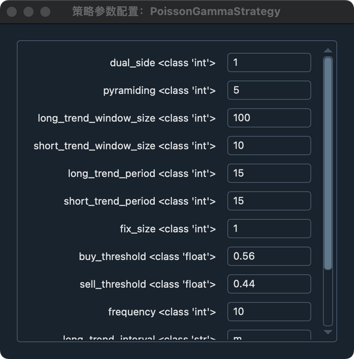
Strategy parameters
- dual_side: whether to open a position in both directions
- pyramiding: maximum number of openings in the same direction
- long_trend_window_size: long period sequence length
- short_trend_window_size: short period sequence length
- long_trend_period: long period granularity,
- short_trend_period: short period granularity
- buy_threshold: long threshold
- sell_threshold: short threshold
- fix_size: the amount of each opening
- frequency: the range of the number of increases
- long_trend_interval:m (m分钟,h小时,d日)
- short_trend_interval:m
Default parameters:
Target: BTCUSD Start date: 2022-1-1 End date: 2023-12-6 Fee rate: 0.002 Funds: 100000
Backtest results
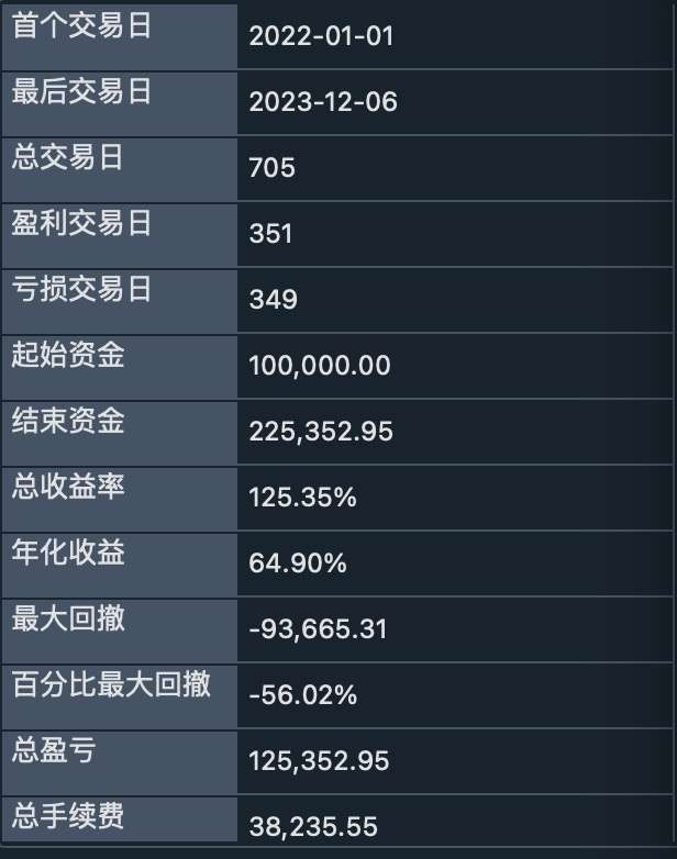
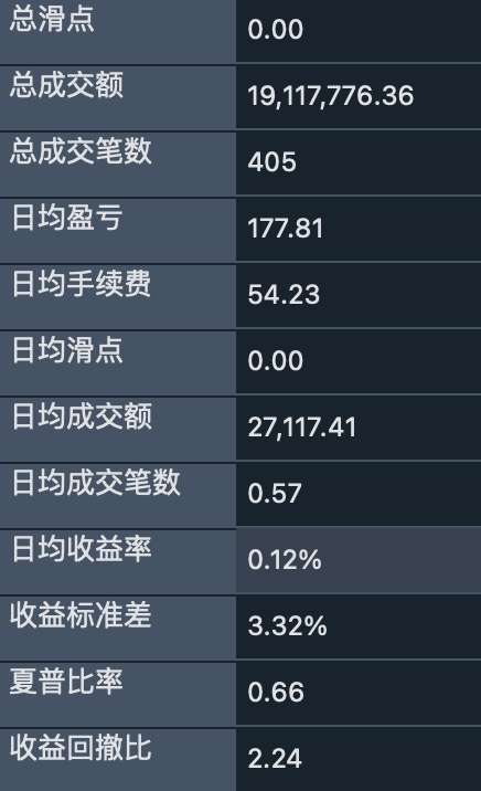
- Strategy curve
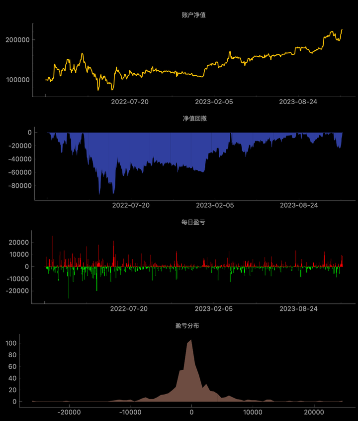
Summary
The Bayesian trading strategy using the gamma-poisson conjugate is very flexible. I only show the backtest results of method 1 in the strategy logic. Readers can also build strategies based on the number of times, rather than converting to probability like me. For example, if the number of posterior increases is 15, can I block the reversal market after 15 increases? Everyone is welcome to discuss.
Strategy code
from vnpy_ctastrategy import (
    CtaTemplate,
    StopOrder,
    TickData,
    BarData,
    TradeData,
    OrderData,
    BarGenerator,
    ArrayManager,
)
import numpy as np
from vnpy.trader.object import Interval
from scipy.stats import gamma, poisson

interval_map = {"m": Interval.MINUTE,
                "h": Interval.HOUR,
                "d": Interval.DAILY}

class PoissonGammaStrategy(CtaTemplate):
    author = "Xuanhao"

    prior = 0
    pyramiding = 1
    frequency = 24
    long_trend_window_size = 5
    short_trend_window_size = 5
    long_trend_period = 1 # 1hour 2hour
    short_trend_period = 5 # 5 minutes
    long_trend_interval = "m"
    short_trend_interval = "m"
    fix_size = 1
    buy_threshold = 0.55
    sell_threshold = 0.45
    dual_side = 1
    parameters = ["dual_side", "pyramiding", "long_trend_window_size","short_trend_window_size","long_trend_period", "short_trend_period" ,"fix_size", "buy_threshold", "sell_threshold", "frequency", "long_trend_interval", "short_trend_interval"]
    variables = ["bayesian_prob"]

    def __init__(self, cta_engine, strategy_name, vt_symbol, setting):
        super().__init__(cta_engine, strategy_name, vt_symbol, setting)
        long_interval = interval_map[self.long_trend_interval]
        short_interval = interval_map[self.short_trend_interval]

        self.bg_long = BarGenerator(self.on_bar, self.long_trend_period, self.on_long_bar, interval=long_interval)
        self.bg_short = BarGenerator(self.on_bar, self.short_trend_period, self.on_short_bar, interval=short_interval)
        self.am_long = ArrayManager(self.long_trend_window_size*self.frequency)
        self.am_short = ArrayManager(self.short_trend_window_size*self.frequency)
        self.priors_inited = False

    def on_init(self):
        self.write_log("策略初始化")
        self.load_bar(10)

    def on_start(self):
        self.write_log("策略启动")
        self.put_event()

    def on_stop(self):
        self.write_log("策略停止")
        self.put_event()

    def on_bar(self, bar: BarData):
        self.bg_long.update_bar(bar)
        self.bg_short.update_bar(bar)

    def on_long_bar(self, long_bar: BarData):
        self.am_long.update_bar(long_bar)
        if not self.am_long.inited:
            return
        poisson_event = []
        for order in range(self.long_trend_window_size):
            ups = sum(1 for index in np.arange((order)*self.frequency, (order+1)*self.frequency, 1) if
                      self.am_long.close_array[index] > self.am_long.open_array[index])
            poisson_event.append(ups)

        mean = np.mean(poisson_event)
        variance = np.var(poisson_event)

        ## MM estimator
        self.alpha_prior = mean ** 2 / variance
        self.beta_prior = mean / variance

        self.priors_inited = True

    def on_short_bar(self, short_bar: BarData):
        self.am_short.update_bar(short_bar)
        if not self.am_short.inited:
            return

        if not self.priors_inited:
            return

        poisson_event = []

        for order in range(self.short_trend_window_size):
            ups = sum(1 for index in np.arange((order) * self.frequency, (order + 1) * self.frequency, 1) if
                      self.am_short.close_array[index] > self.am_short.open_array[index])
            poisson_event.append(ups)

        self.alpha_post = self.alpha_prior + sum(poisson_event)
        self.beta_post = self.beta_prior + self.short_trend_window_size

        # use posterior mean or mode
        self.poster_mean = self.alpha_post/self.beta_post
        self.poster_var = self.alpha_post/(self.beta_post)**2
        self.poster_mode = (self.alpha_post-1)/self.beta_post

        if self.dual_side:
            # both long and short
            if self.poster_mode/self.short_trend_window_size > self.buy_threshold:
                if self.pos >= 0:
                    if abs(self.pos) < self.pyramiding:
                        self.buy(short_bar.close_price, self.fix_size)
                else:
                    self.cover(short_bar.close_price, abs(self.pos))
                    self.buy(short_bar.close_price, self.fix_size)


            if self.poster_mode/self.short_trend_window_size < self.sell_threshold:
                if self.pos <= 0:
                    if abs(self.pos) < self.pyramiding:
                        self.short(short_bar.close_price, self.fix_size)
                else:
                    self.sell(short_bar.close_price, abs(self.pos))
                    self.short(short_bar.close_price, self.fix_size)

        else:
            if self.poster_mode/self.short_trend_window_size > self.buy_threshold:
                if self.pos >= 0 and self.pos < self.pyramiding:
                    self.buy(short_bar.close_price, self.fix_size)

            if self.poster_mode/self.short_trend_window_size < self.sell_threshold:
                if self.pos != 0:
                    self.sell(short_bar.close_price, self.pos)