Journey to a universal hedge system

Intro

Statistical arbitrage or hedging has already been known for a long time, people usually tackle this trading strategy with models that have strong assumptions, and generally have only limited amount of asset pairs to trade based on the some macro or micro economics assumption.

In this essay, we want to explore more modern and diverse statistical method or machine learning methods for hedging. We will address two questions:

1. Is it possible to find arbitrage opportunities for any given paris ?
2. What models are suitable for arbitrage ?

What is hedging?

Hedge is about longing and shorting an asset or different asset at the same time, aiming to lower the risk and harvest profit when the opportunity arises.

What do we need to estimate for a hedging system?

For a hedging stratey to run properly, we need to define the Hedge ratio. It’s the ratio of long positions to short positions. Usually it’s define by expertise or a linear regression model. In this essay we will try out other methods.

An heuristic example

In finance, people who holds the spot position can choose to short its futures counterpart to preserve its value. If we have bitcoin spot, but we want to lower the risk of holding the spot, we short selling its BTC futures contract in the next season, and since price of the spot and the price of the futures will converge at the delivery date as the graph show below, 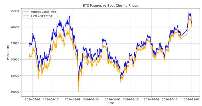we basically lock in the value of the spot the moment we short selling its future. 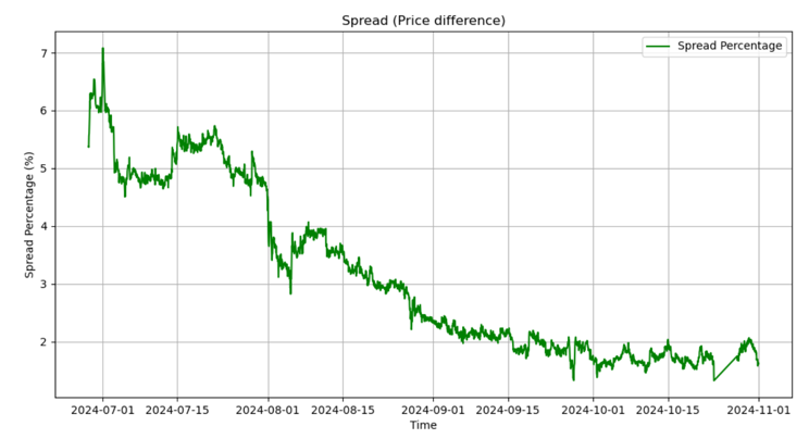In this example the price difference (spread) is calculated by:

$$ spread_t = future_t - spot_t $$

The Basis Percent is calculated by:

$$ Basis = (future_t - spot_t)/spot_t $$

And from this data the maximum basis is around 7%, so the maximum profit that we can yeild here is 3.5% since we need to split the position for equally for two assets.

And heuristically we get a ‘pesudo regression model’ :

$$ future_t = spot_t + spread_t $$

The slope $\beta$ in this model is the hedge ratio and it’s currently defined as 1. But we are ‘cheating’ here since we know that the futures and spot price will converge (for the same asset btc). Remember that our goal is to find an universal hedge system, which means we don’t want to just limit ourselves to do hedging within the same asset, we want to find opportunities between different assets. Ideally, we want to find hedging opportunities given any pair of assets. Nautrally, we need a more complex model to define the hedge ratio based on the historical data.

What assumptions do we need?

The first assumption is that the two assets that you try to hedge need to have a cointegrated relationship at least in some period.

Cointegration

Now let’s talk about one of the most important concept in hedging. What is cointegration? Stock price, interest rate etc. time series in finance, are usually assumed to be a random walk process.

$$ X_t = X_{t-1} + \epsilon_t, \quad \epsilon_t \sim \mathcal{N}(0, \sigma^2) $$

and if $Y_t$ is induced from this random walk $X_t$by:

$$ Y_t = \beta X_t + \mu + q_t $$

We can say this two random walk process is cointegrated where $q_t$ can be any kind of stationary process, such as AR(1). And the $\beta$ define their long term equilibrium relationship.

Is cointegration important for hedging?

Yes! remember we were trading based on the difference between two assets? If the residual of of that ‘pesudo regression’ model is stationary, then we can make a line to define (such as one standard deviation) the target profit we want.

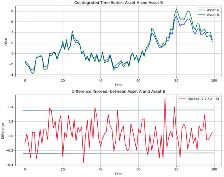
As the graph shows, the hedge ratio is 1.2, if the residual is stationary (having constant mean, not nessarily constant variance) then everytime it reaches our target profit line we can open the position, when it revert back to mean then we can close the position.

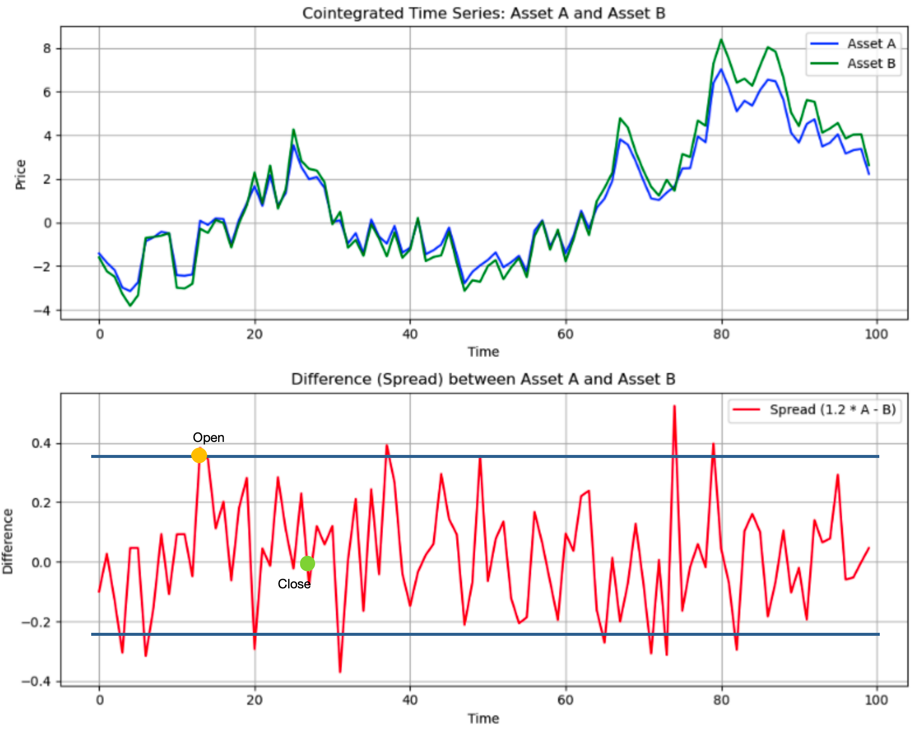
So the fact that the residual is stationary is our ideal trading scenario! what’s more, the residual can be heteroskedasiticity. In fact, the higher the standard deviation it has, the higher the profit we yield.

(The graph from the non-linear cointegratioin paper)

But modeling heteroskedasiticity is definetly another challenage, we will address this problem later.

Is this assumption too strong ?

It certianty is, since the market is an ever changing environment. So it would be more reasonable to assume that the $\beta$ is time verying, or better, all components in the regression model to be time verying:

$$ Y_t = \beta_t * Xt + \mu_t + \epsilon_t $$

we can assume that $\beta$ and $\mu$ to be a Hidden markov model in which you can choose how many regeims you want to switch. We can also assume that they are random walks:

$$ \beta_t = \beta_{t-1} + \eta_{\beta,t}, \quad \eta_{\beta,t} \sim \mathcal{N}(0, \sigma_{\beta}^2) $$$$ \mu_t = \mu_{t-1} + \eta_{\mu,t}, \quad \eta_{\mu,t} \sim \mathcal{N}(0, \sigma_{\mu}^2) $$

What model can we use

After discussing the assumption, we know that our motivation is to find a regression model that has time verying component. The model is unsupervised since we can’t observe what’s the real value of each component.

The model should decompose a non-stationary time series into two explainable latent variable :

• The regression part $\beta_t$ scaled by another time series: $\beta_t X_t$
• The stochastic trend part: $\mu_t$

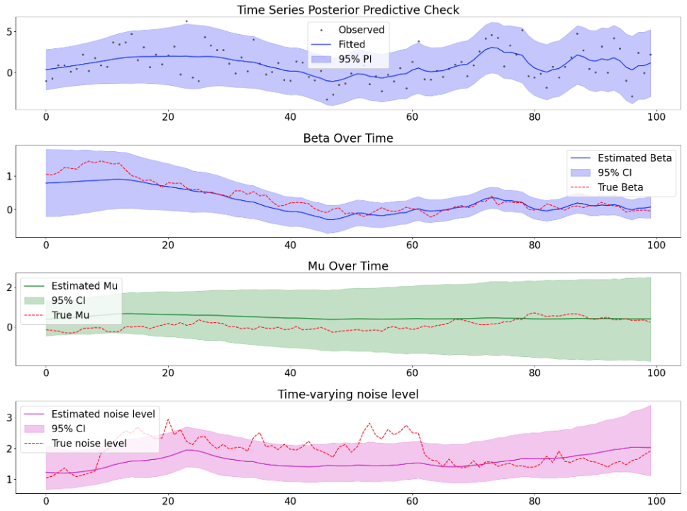
Simulation study

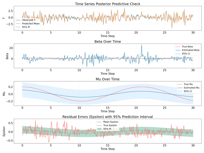
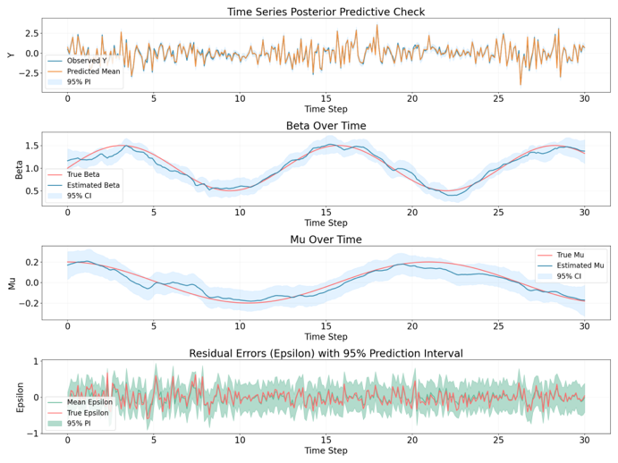
In order to test if the model can filter the signal well, we need to do simulation where the true value of each component is known,

Rolling window regression

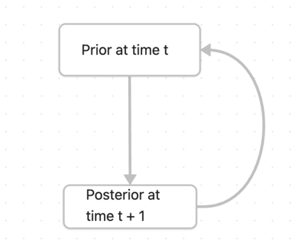
For adaptiing the ever changing market environment, we can give the model a rolling window to get the time verying parameter. If the step size is one then we can have a new parameter after observing every new time step. But if we fit the new model after every time step, it’s likely that we lost the information from the last time step. So in order to adapt the environment but still take the past into consideration, we can use Bayesian regression with recursive prior.

Bayesian regression

Since the data from the market is a data stream, we can use bayesian recursive prior updating everytime we get new information:

Bayesian Generalized additive model

We can give a different feature representation to each component and sum up together, such as a polynoimal function with higher degree. The formula:

$$Y_t = \beta(t)X_t + \mu(t) + \varepsilon_t$$$$\varepsilon_t \sim \mathcal{N}(0,\sigma^2)$$

The likelihood:

$$P(Y|\beta, \mu, \sigma^2) = \prod_t \mathcal{N}(Y_t|\beta(t)X_t + \mu(t), \sigma_t^2)$$

The additive component:

$$\beta(t) = B(t)b$$$$\mu(t) = B(t)m$$$$Y_t = X_t B(t)b + B(t)m + \varepsilon_t$$

The prior:

$$b \sim \mathcal{N}(0, \lambda^{-1}I)$$$$m \sim \mathcal{N}(0, \lambda^{-1}I)$$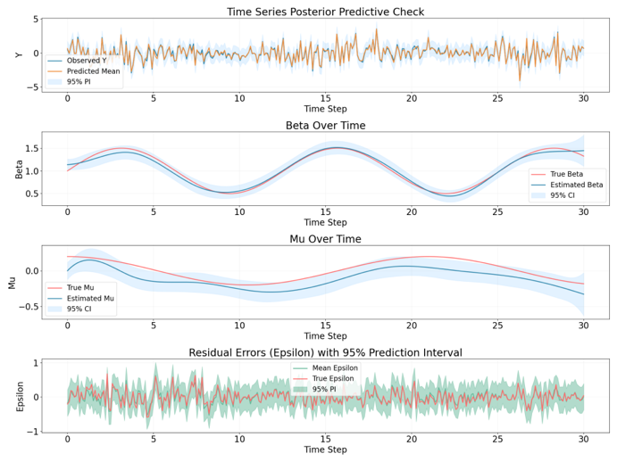

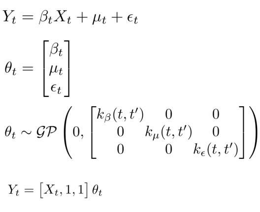
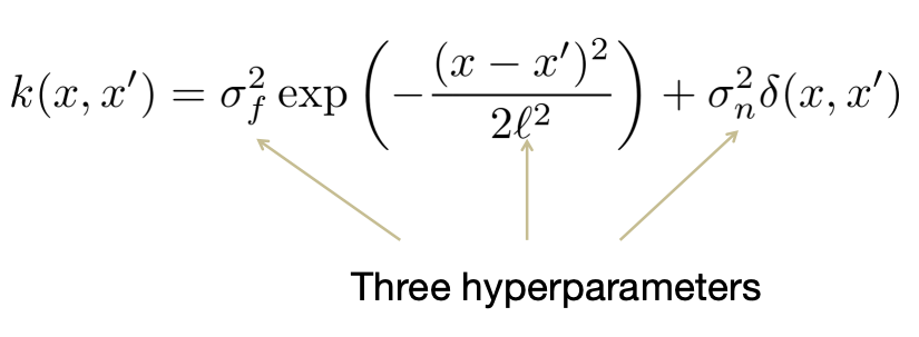
Composite Gaussian Process

We use a dedicate kernel for each component in the regression model. The parameter itself follows a composite Gaussian Process prior. we update the prior by maximizing the likelihood.

Bayesian Structural Time Series

Bayesian structural time series model is a flexible model that can decompose the time series into explainable properties. We can incorperate different prior distribution for modeling the time verying component. Like I said before the time verying natural can each component can be a HMM or a random walk etc: Hidden Markov model prior(two regime) 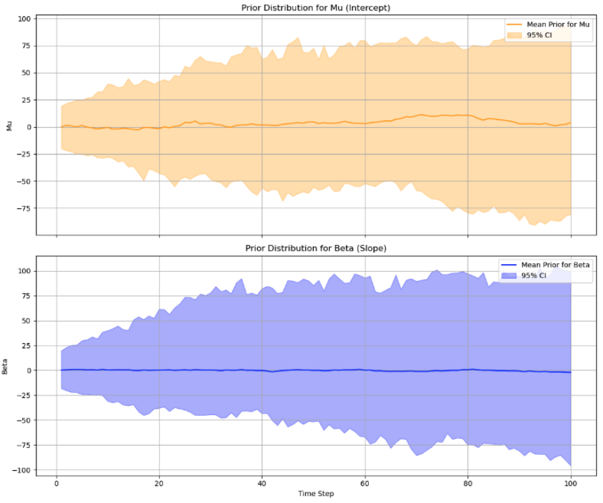Gaussian Random walk prior：

$$\beta_{t+1} | \beta_t, \sigma_\beta^2 \sim \mathcal{N}(\beta_t, \sigma_\beta^2)$$$$\mu_{t+1} | \mu_t, \sigma_\mu^2 \sim \mathcal{N}(\mu_t, \sigma_\mu^2)$$$$Y_t | \beta_t, \mu_t, \sigma^2 \sim \mathcal{N}(\beta_t X_t + \mu_t, \sigma^2)$$$$\sigma^2, \sigma_\beta^2, \sigma_\mu^2 \sim \text{Half-Cauchy}(0, 1)$$

What’s more, we can also give a heterogeneity prior to the random noise level:

$$\log \sigma_t \sim \mathcal{N}(\log \sigma_{t-1}, 0.1^2)$$$$\log \sigma_1 \sim \mathcal{N}(0, 1)$$$$\sigma_t = \exp(\log \sigma_t)$$

Real world data experiment

In this section we will investigate if the models can decompose the time series well. But firstly we need to find potentially cointegration pairs. we wanna have pairs that shares common trend at least in some period. To model this non-linear relationship, we can use Gaussian process to handle.

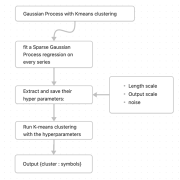
Finding cointegration pairs using Sparse GPs

Because our time series are really long around 2000 time points, and the cointegration is a long term relationship, we want to have a model that can capture this kind of non-linear correlation behavior but also without having much computational complexity. Having said that Sparse GPs is the first choice. We can use it to do the clustering in the following way: After clustering using all the stocks from Sp500 data, the algorithm did find stocks that behave the same: 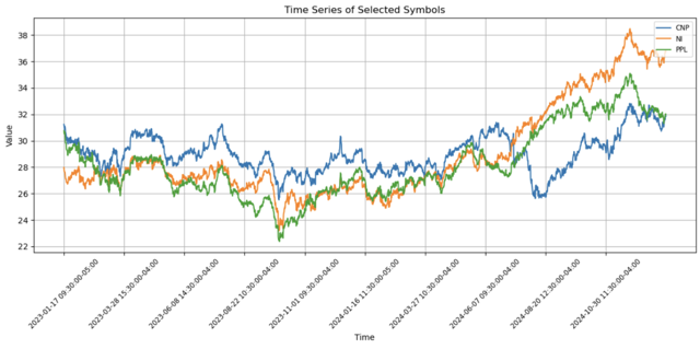The similar stock behavior of CenterPoint Energy, NiSource Inc., and PPL Corporation is likely due to their shared roles in the utility sector, subjecting them to comparable regulatory frameworks and market influences.

Question before the experiment

Question is:

We can’t know the true value of latent variable

Answer:

1. Evaluate if the model can decompose the signal into time verying components

2. Evaluate if the residual has mean reverting behavior after ‘filtering’

Experiment result (stock pairs NI and PPL)

Bayesian regression

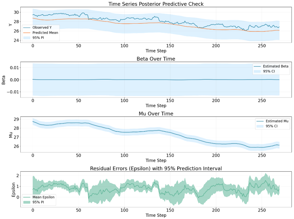The residual does have certaint level of mean reverting behavior but seems to have small trending behavior from time to time.

Bayesian GAM

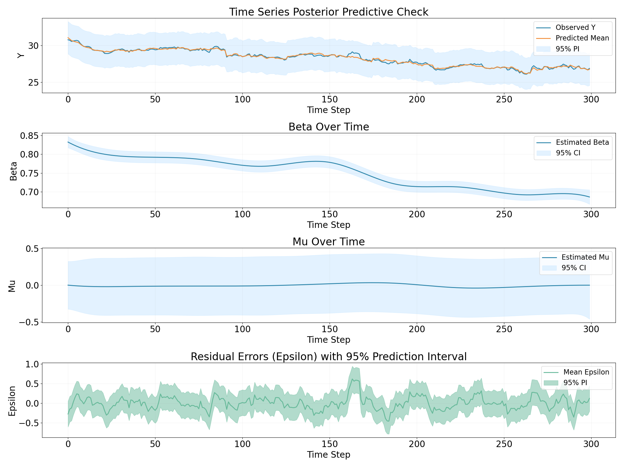The decomposition result of GAM model seems to be the counterpart of the bayesian regression model. However, that’s an expected behavior since the function $Y_t = \beta_t * Xt + \mu_t + \epsilon_t $ can have multiple solution. And the fluctuation of residual is smaller comparatively.

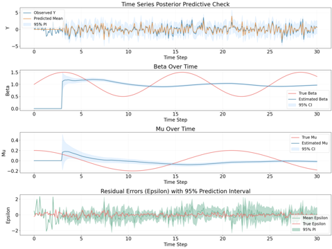
Composite Gaussian Process

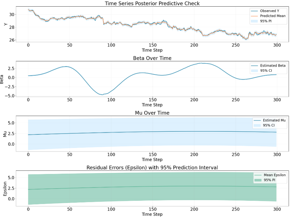The decomposition from GPs behaves differently from other three algorithm and notice that the Epsilon part is a prediction not the real residual, so by using composite GPs we can have a prediction of the range of residual. (but here might be improved by restrict it to have zero mean, so that all other variation of the data would be captured by other two components)

BSTS with heteroskedasticity

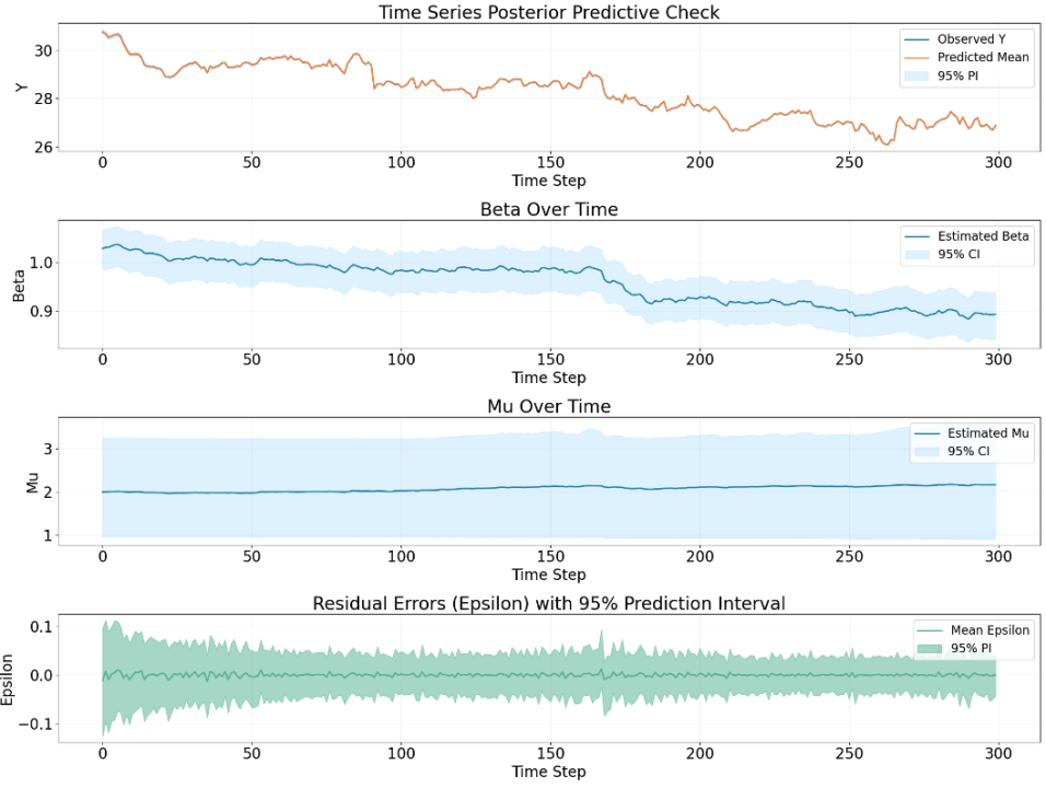The residual of BSTS model looks the most stationary, but it seems that the fluctuation is too small to generate profit, the model is overfitting to a degree that the time series is decomposed ’too well’, the residual becomes tiny, so it’s hard to generate high profit with this residual, but if you have low trading fee it would possibly still work since the trading frequency is really high.

Summary

Whether a model is good for developing trading strategy depends on how does the residual of the model behave. It’s a bargain between

Big residual, low frequency mean reverting and

small residual but high frequency mean reverting.

In the real world scenario, choosing which kind of model depends on the trading fee and the latency of the server.

In the next chapter, we are going to explore these models in a backtesting environment.