Journey to a universal hedge system (part 2)

In the previous post we have talked about the implementation of models in pairs trading and their experiment, now let’s try these strategies out using a backtesting framework.

Model budget analysis

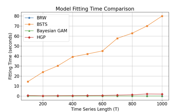Notice that the BSTS model has o(n) computation complexity. Other models have negligible complexity level.

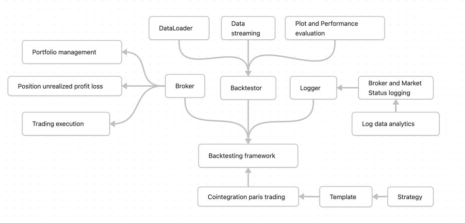
Backtesting framework

The backtesting frame uses simple object-oriented programming structure.

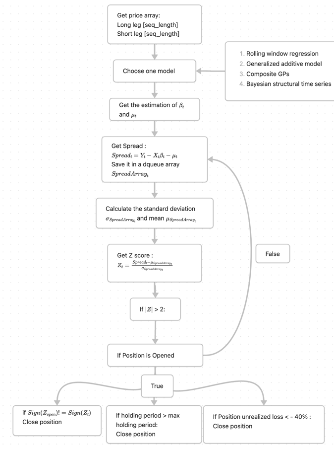
Strategy flow chart

The strategy can multiple exit position options to prevent high drop down.

Paris selection

In the previous post we have introduced the sparse gaussian process clustering method, and here are the clusters the algorithm found using the Sp500 as dataset: 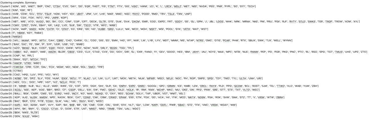And I choosed cluster 1 and 24 here, since we are going to use every single pair in the cluster so to facilitate the experiment I chose the cluster that’s not too large.

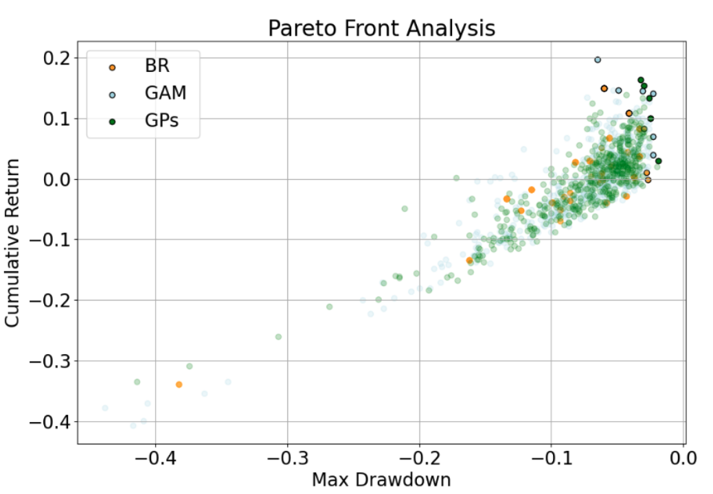
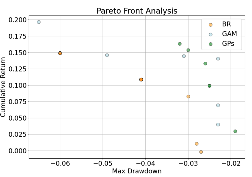
Pareto front analysis

During the experiment, because we have to refit the model after one step size. It’s too time consuming to refit the BSTS model so its experiment couldn’t be finished. For the multi objective

Backtest cluster:

‘ADM’, ‘AIG’, ‘ANET’, ‘BXP’, ‘CNC’, ‘CTSH’, ‘CVS’, ‘DAY’, ‘DD’, ‘EQR’, ‘FAST’, ‘FIS’, ‘FTNT’, ‘FTV’, ‘GIS’, ‘HSIC’, ‘HWM’, ‘JCI’, ‘K’, ‘L’, ‘LRCX’, ‘MDLZ’, ‘MET’, ‘NEE’, ‘NVDA’, ‘PEG’, ‘PNR’, ‘PYPL’, ‘SO’, ‘SYY’, ‘TECH’

Backtest cluster:

‘BALL’, ‘BSX’, ‘CARR’, ‘CMS’, ‘ES’, ‘EVRG’, ‘HAS’, ‘INCY’, ‘KO’, ‘MAS’, ‘NDAQ’, ‘O’, ‘OXY’, ‘REG’, ‘SCHW’, ‘SOLV’, ‘TAP’, ‘UBER’, ‘VST’, ‘WMT’, ‘XEL’

Model comparison

Metric	Model	Min	Q25	Median	Q75	Max
Cumulative Return	BR	-0.338	-0.033	0.003	0.037	0.149
	GAM	-0.406	-0.045	-0.003	0.034	0.197
	GPS	-0.334	-0.043	0.001	0.030	0.163
Annualized Volatility	BR	0.013	0.016	0.018	0.024	0.061
	GAM	0.008	0.014	0.017	0.021	0.056
	GPS	0.008	0.014	0.016	0.020	0.053
Sharpe Ratio	BR	-0.455	-0.125	0.021	0.160	0.618
	GAM	-0.770	-0.179	-0.008	0.170	0.819
	GPS	-0.778	-0.182	0.015	0.157	0.763
Max Drawdown	BR	-0.382	-0.093	-0.062	-0.043	-0.027
	GAM	-0.438	-0.095	-0.063	-0.049	-0.023
	GPS	-0.414	-0.091	-0.062	-0.046	-0.019

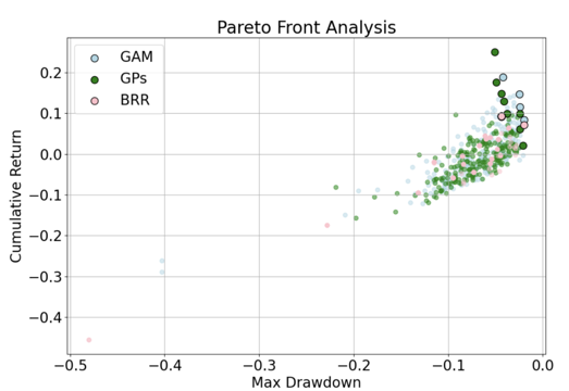
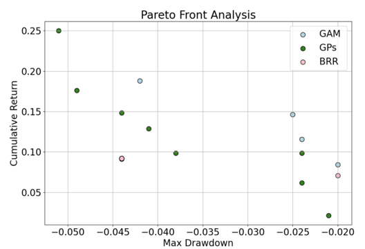
Metric	Model	Min	Q25	Median	Q75	Max
Cumulative Return	BR	-0.455	-0.025	-0.003	0.038	0.092
	GAM	-0.290	-0.048	-0.011	0.036	0.188
	GPs	-0.157	-0.048	-0.012	0.022	0.250
Annualized Volatility	BR	0.008	0.014	0.016	0.021	0.071
	GAM	0.005	0.013	0.016	0.019	0.057
	GPs	0.007	0.013	0.016	0.018	0.033
Sharpe Ratio	BR	-0.634	-0.117	-0.004	0.203	0.658
	GAM	-0.783	-0.217	-0.051	0.223	1.119
	GPs	-0.767	-0.230	-0.052	0.124	0.867
Max Drawdown	BR	-0.480	-0.085	-0.060	-0.047	-0.020
	GAM	-0.403	-0.090	-0.066	-0.042	-0.020
	GPs	-0.219	-0.089	-0.067	-0.046	-0.021

Future works

Find quick online updating methods for BSTS and GPs.

• Sherman–Morrison formula
• Woodbury formula

Run simulation for BSTS using paper trading API

Change other model to also adapt to the heteroskedasticity

The strategy still has to be tuned

• The max holding period
• stop loss
• window size
• ADF test P value
• Position amount ….

Run simulation on crypto currency data and make a comparsion.