The wavelet transform is a signal processing tool applicable to both images and time series. The figure below illustrates an example of its application in image processing, where it decomposes an image into multiple frequency channels to achieve signal decomposition and compression. For instance, JPEG 2000 is an image compression standard based on the wavelet transform (https://zh.wikipedia.org/wiki/JPEG_2000):
Wavelet Transform Applied to Image Processing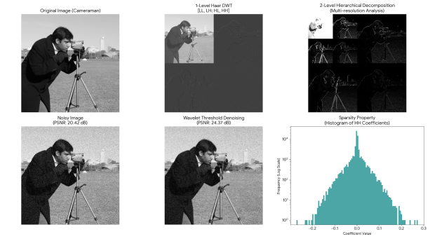
Comparison Between Wavelet Transform and Fourier Transform
As a signal processing tool, we must inevitably mention another common tool: the Fourier transform. First, let me explain the similarities and differences between Fourier transform and wavelet transform. Imagine we’re observing a traffic light. We know that a traffic light has three colors (red, yellow, green) and changes according to a certain pattern:
Figure 1: Traffic Light Example
In contrast, from the wavelet transform result in Figure 1 (at the bottom), with the vertical axis representing frequency and the horizontal axis representing the time when each frequency appears, we can determine that red appears first, then yellow, and finally green. Why does this difference occur? The following will explain it from theory to application.
Orthogonal Basis and Dot Product
The essence of signal processing is basis transformation. The Fourier transform projects a signal onto a set of orthogonal complex exponential basis functions: cos + i*sin. By calculating the inner product of the signal with basis functions of different frequencies, we can obtain the component weights of the signal at various frequencies, thereby analyzing the spectrum characteristics of the signal:
Figure 2: Orthogonal Basis at Different Frequencies ω
Mother Wavelet and Father Wavelet
On the other hand, wavelet transform uses a series of functions that are only locally non-zero to compute inner products with the original signal. We call this locally non-zero function the mother wavelet. Scholars have defined various shapes of mother wavelets to extract different types of information. Here are some examples:
Figure 3: Various Mother Wavelets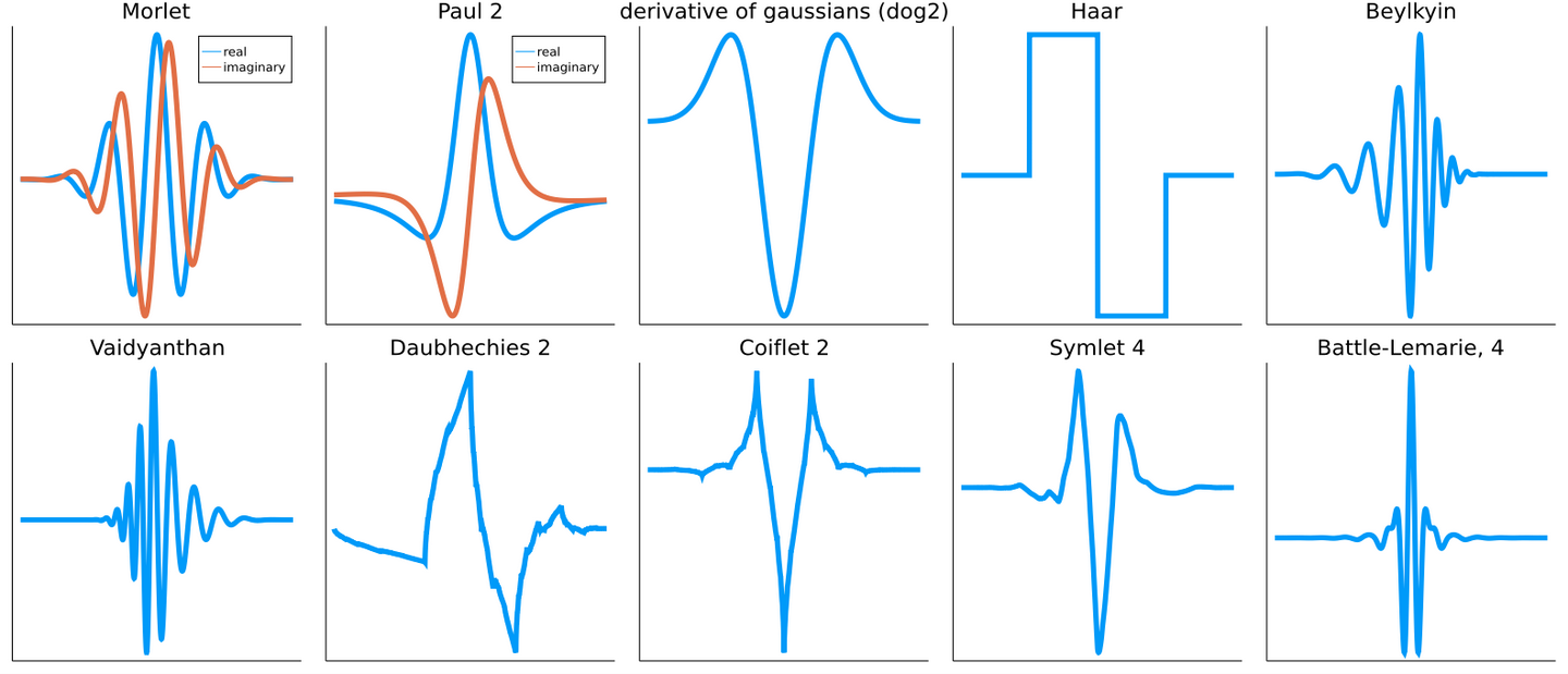
Figure 4: Scanning Signal with Wavelet
Figure 5:Scaling the Wavelet
Figure 6: Multi-scale Wavelet Components
Figure 7: Wavelet Scalogram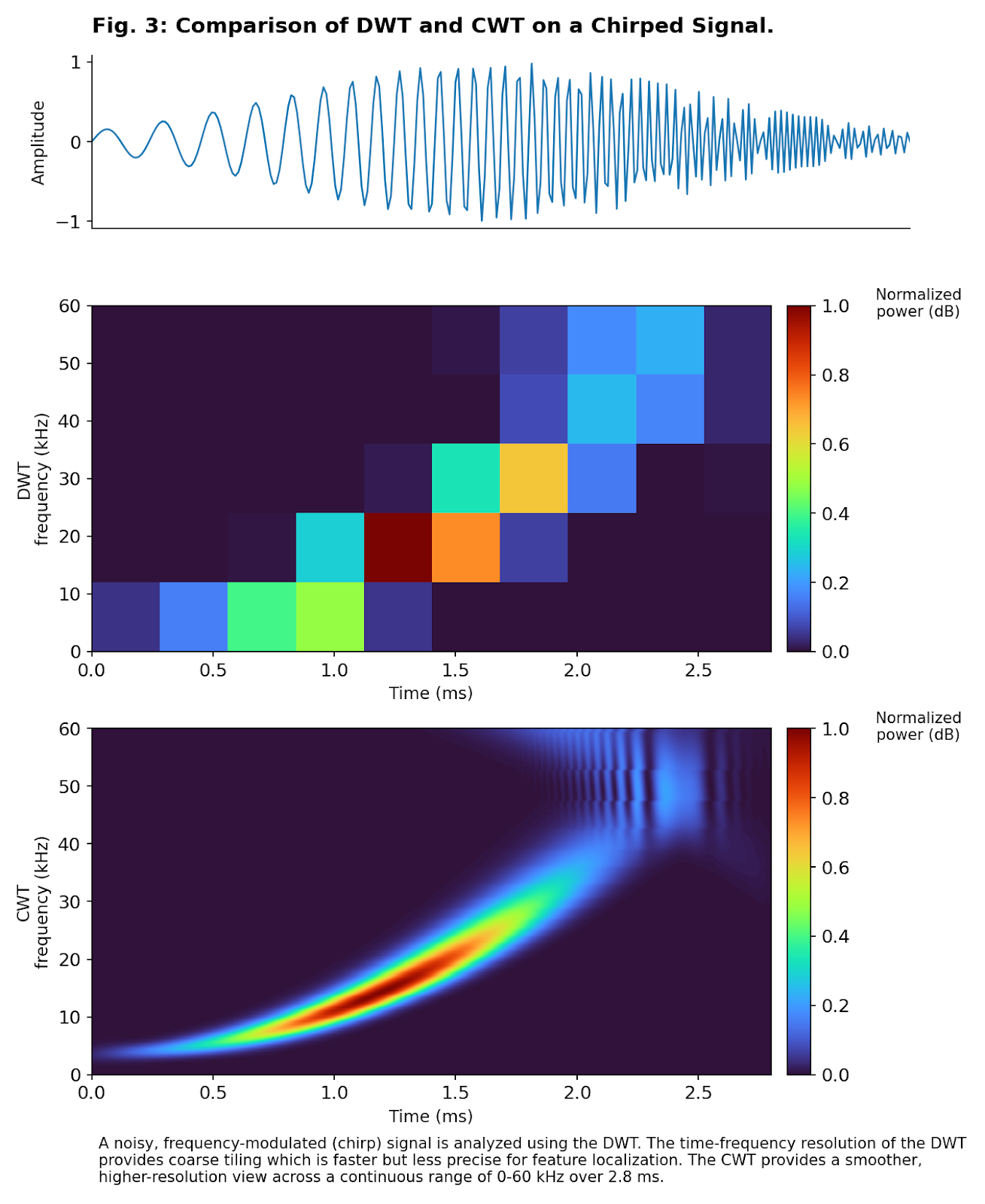
Wavelet Transform Feature Extraction
In machine learning, we generally use the Discrete Wavelet Transform (DWT) because the Continuous Wavelet Transform (CWT) is redundant and can easily cause machine learning algorithms to learn noise. The figure below is an example of the application of discrete wavelet transform in time series modeling:
Figure 8: Discrete Wavelet Transform Example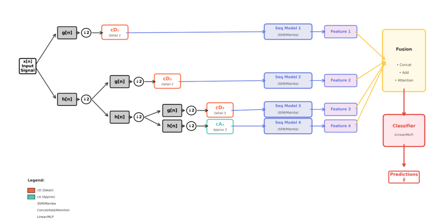
The result of the low-pass filter is further decomposed by the same pair of high-pass and low-pass filters. Each layer of wavelet transform downsamples the signal to achieve multi-resolution analysis. We can also see that the coefficients from each layer are connected to the machine learning algorithm, rather than using only the last layer’s coefficients, which can be seen as a form of skip connection. It’s worth noting that we can either choose predefined wavelet families from Figure 3, or let the machine learning algorithm learn the wavelet family itself.
A standard wavelet family must satisfy a series of conditions, such as perfect reconstruction, orthogonality, discreteness, and uniform energy. We can incorporate these conditions into the loss function of learnable wavelets. After training the wavelets, we freeze their weights and continue training downstream tasks, which can be seen as two-stage training.

Figure 9: Learnable Wavelet Example
It’s worth mentioning that wavelet training can be simplified to only training the high-pass filter, while the low-pass filter can be calculated using the Quadrature Mirror Filter formula. It’s not actually a sophisticated algorithm; it simply means lowering the frequency of the high-pass filter to directly obtain the low-pass filter, and finally ensuring their frequencies don’t overlap:
Figure 10: Quadrature Mirror Filter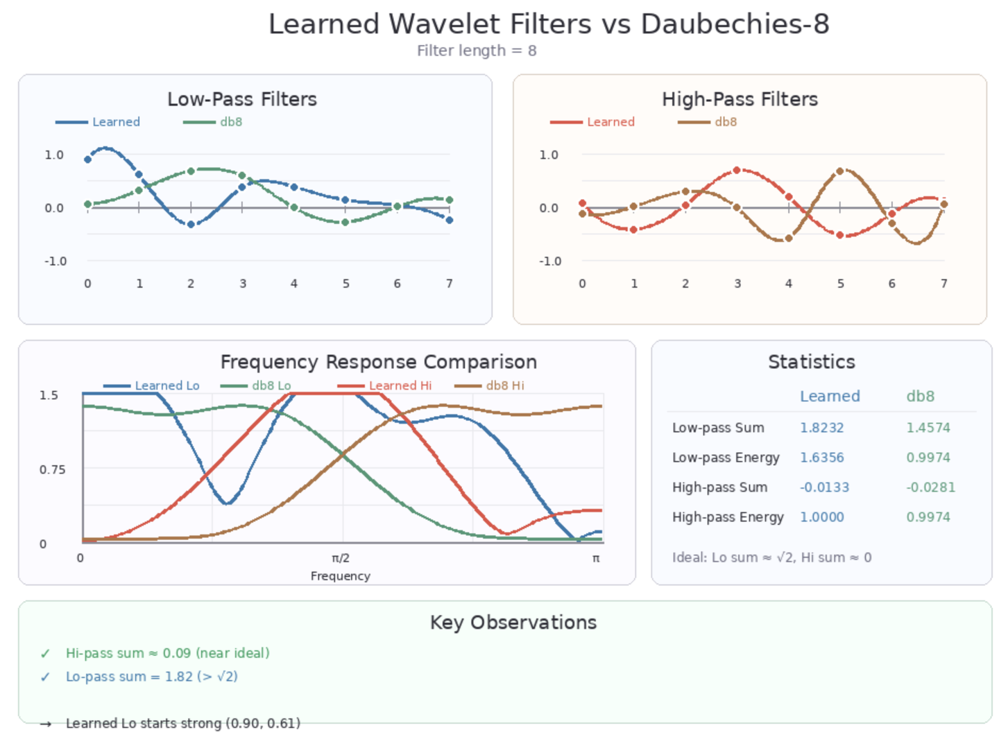
Program Implementation
In Python, PyWavelets (https://pywavelets.readthedocs.io/en/latest/install.html) provides a complete wavelet transform library. Of course, if you’re using learnable wavelets, you can use the following methods for computation:
- First, generate the analysis matrix (N×N) you need based on the signal length N (a matrix containing function values of wavelet filter banks at different positions):
- Multiply the original signal (1×N) with this analysis matrix
- Downsample the resulting (1×N) vector until you reach your desired number of levels
- Perform inverse wavelet transform using the obtained coefficients multiplied by the transpose of the analysis matrix (because the inverse of a matrix composed of orthogonal basis is exactly its own transpose, which is one of the benefits of choosing orthogonal bases), then upsample until the length matches the original data.
- Calculate the reconstruction error between the signal obtained from the inverse transform and the original signal, then backpropagate.
Below, let’s see what an analysis matrix of length N=32 looks like:
Figure 11: Analysis Matrix Example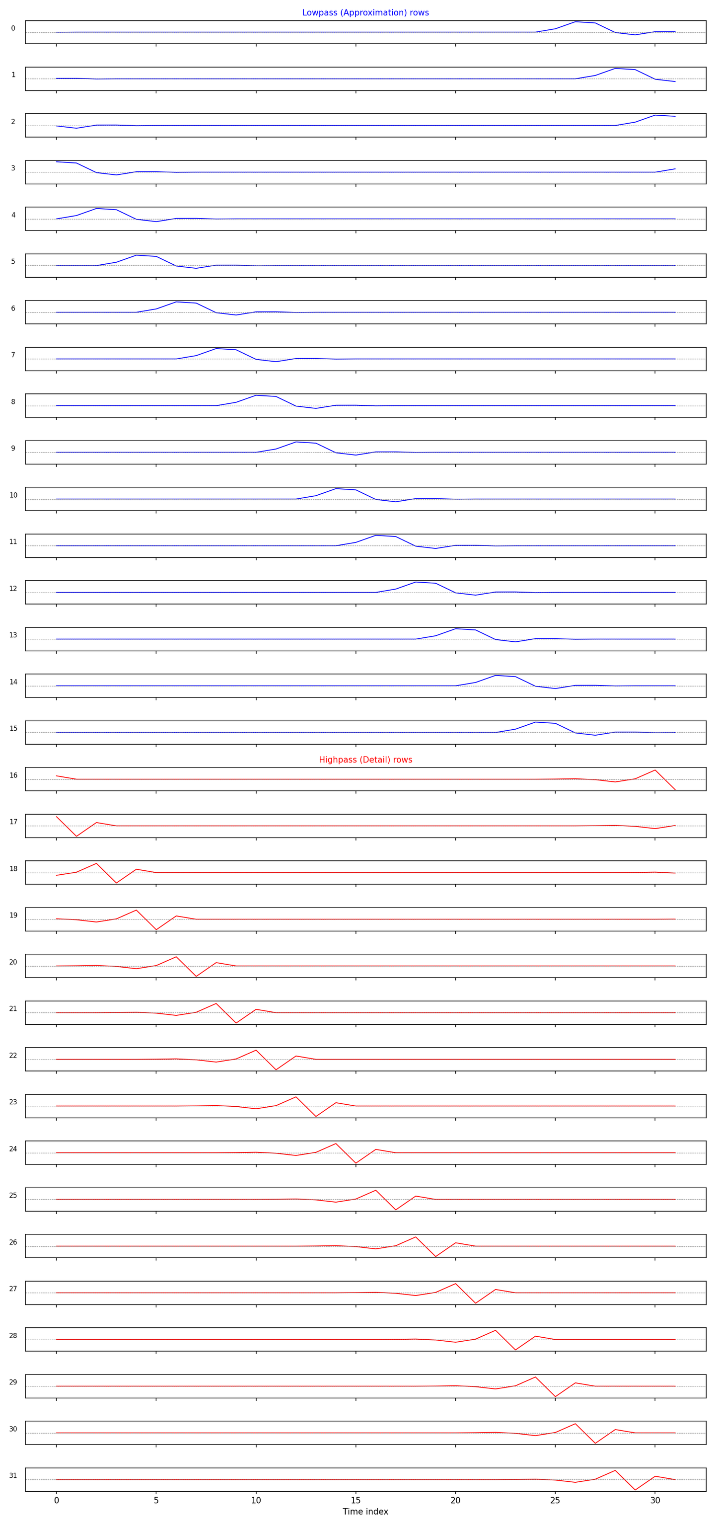
Figure 12: Reconstruction Results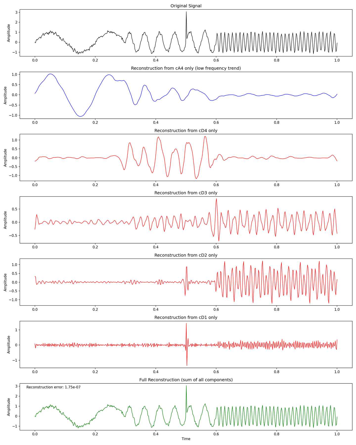
Figure 13: Position Information from Wavelet
Bonus:
- The results of wavelet transform usually require some feature engineering to be effective.
- Learnable wavelets for feature extraction are not necessarily better than custom wavelets.
- Wavelet transform is, to some extent, CNN + regularization.
Welcome to discuss wavelet transform and related theory with me!
Classic Literature on Signal Processing and Wavelet Analysis
Mallat, S. A Wavelet Tour of Signal Processing: The Sparse Way. Academic Press, 2008 (3rd Edition).
Vaidyanathan, P. P. Multirate Systems and Filter Banks. Prentice Hall, 1993.
Daubechies, I. Ten Lectures on Wavelets. Society for Industrial and Applied Mathematics (SIAM), 1992.